Chapter 3
Descriptive Statistics: Numerical Measures
Case Problem 1: Pelican Stores
1. Descriptive statistics for all customers are shown followed by the same descriptive statistics for 4
subgroups of customers.
Net Sales (All Customers)
Mean
$77.60
Median
$59.71
Std. Dev.
$55.66
Range
$274.36
Skewness
1.715
NET SALES BY CUSTOMER TYPE
Married
Single
Regular
Promotion
Mean
$78.03
$77.04
$61.99
$85.25
Median
59.00
69.00
51.00
63.64
Std. Deviation
57.67
46.21
35.07
61.38
Range
274.36
163.30
137.25
274.36
Skewness
1.732
1.254
1.351
1.520
A few observations can be made:
a. Customers taking advantage of the promotional coupons spent more money on average. The mean
amount spent by all customers is $77.60; the average amount spent by promotional customers was
$85.25.
There are many other descriptive statistics students may generate using the other variables. These
will lead to other observations concerning the demographics of the Pelican customers and their
buying behavior. For example, the following crosstabulation shows data for the 70 female customers
classified by type of customer and marital status.
Gender
Marital Status
Female
Female Total
Grand Total
Type of Customer
Data
Married
Single
Promotional
Average of Age
44
33
43
43
Average of Net Sales
86.48
75.96
85.20
85.20
Count of Customer
58
8
66
66
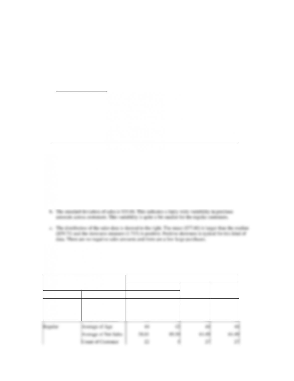
Regular
Average of Age
44
42
44
44
Average of Net Sales
58.81
89.50
64.49
64.49
Count of Customer
22
5
27
27
Total Average of Age
44
36
43
43
Total Average of Net Sales
79
81
79
79
Total Count of Customer
80
13
93
93
We see that for the 58 female-married promotional customers the average net sales was $86.48, and
that for the 8 female-single promotional customers the average net sales was $75.96. Thus, for the
2. The correlation coefficient for the association of sales with age is r = .01. There does not appear to
be any relationship between net sales and age.
Case Problem 2: The Motion Picture Industry
This case provides the student with the opportunity to use numerical measures to continue the analysis of
the motion picture industry data first presented in Chapter 2. Developing and interpreting descriptive
statistics such as the mean, median, standard deviation and range are emphasized. Five-number summaries
and the identification of outliers are also of interest. Interpretations and insights can vary. We illustrate
some below.
Descriptive Statistics
Descriptive Statistics provided by Excel follows:
Opening Gross Sales
($millions)
Total Gross Sales
($millions)
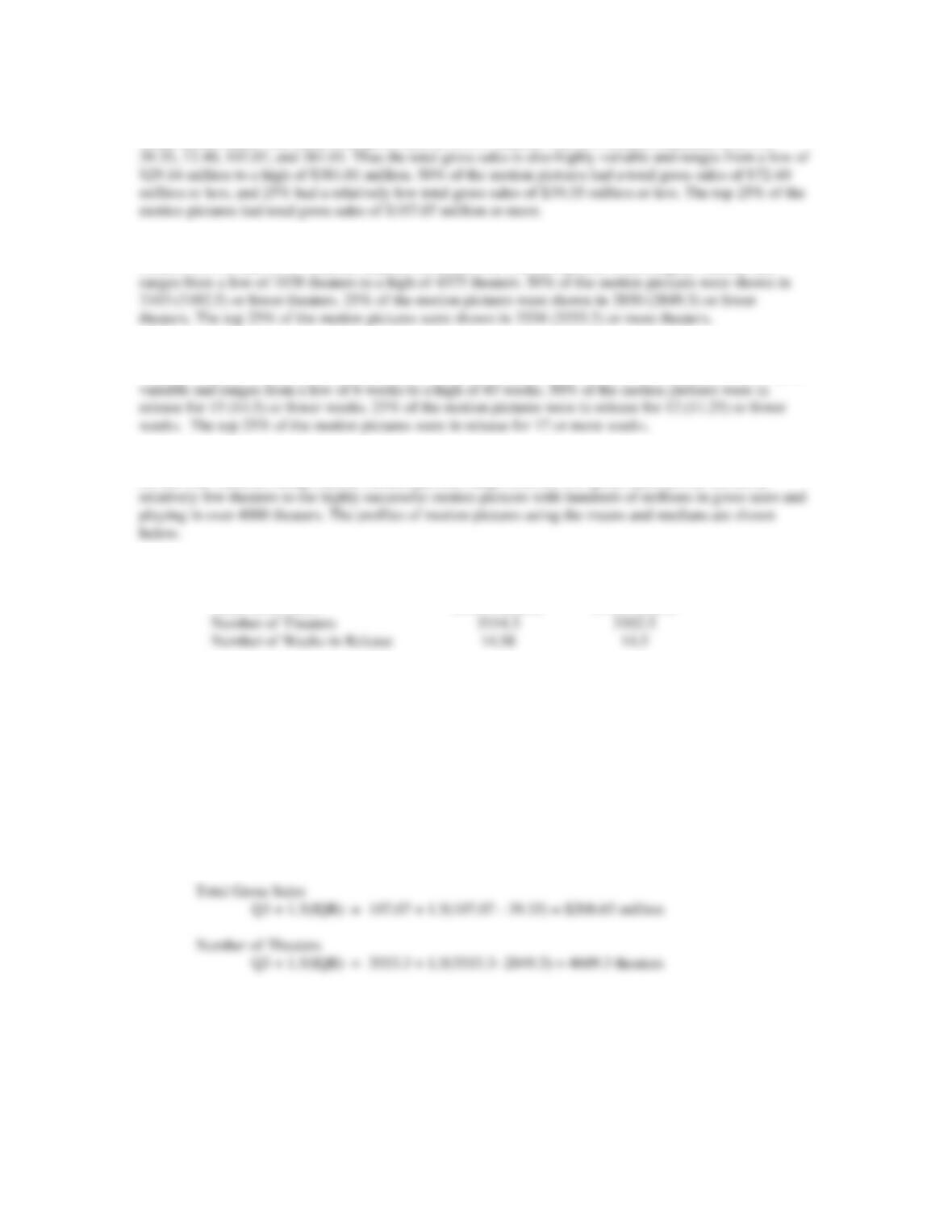
Number of
Theaters
Weeks in
Release
Mean
27.51
90.47
3114.35
14.58
Standard Error
2.65
6.81
61.08
0.50
Median
19.08
72.4
3102.5
14.5
Mode
#N/A
37.3
3555
16
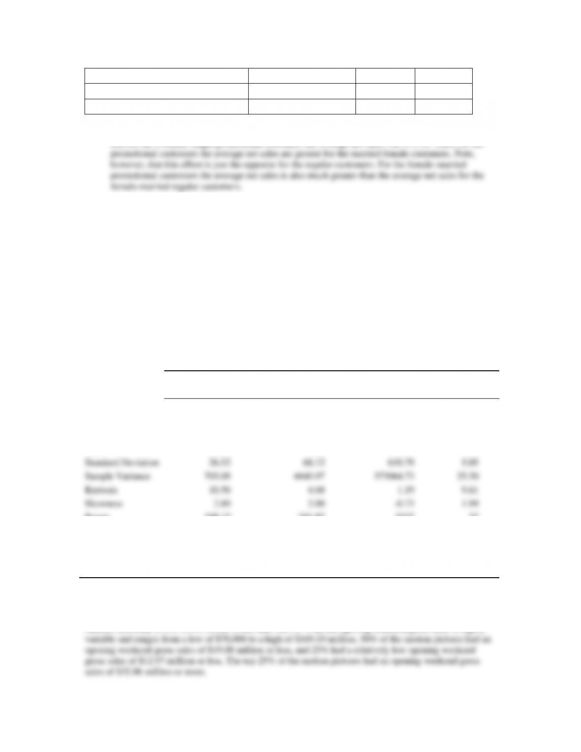
Standard Deviation
26.52
68.12
610.79
5.05
Sample Variance
703.08
4640.97
373064.73
25.50
Kurtosis
10.56
4.68
1.19
9.61
Skewness
2.89
2.00
-0.73
1.99
Range
169.12
351.87
3337
37
Minimum
0.07
29.14
1038
6
Maximum
169.19
381.01
4375
43
Sum
2751.49
9046.64
311435
1458
Count
100
100
100
100
Interpretation
Opening Weekend Gross Sales. The mean opening weekend gross sales is $27.51 million. The five-
number summary is .07, 12.97, 19.08, 32.06, and 169.19. Thus the opening weekend gross sales is highly
Total Gross Sales. The mean total gross sales is $90.47 million. The five-number summary is 29.14,
Number of Theaters. The mean number of theaters is 3114.3. The five-number summary is 1038, 2849.3,
3102.5, 3553.3, and 4375. Thus the number of theaters for a motion picture is also highly variable and
Number of Weeks in Release. The mean number of weeks in release for motion pictures is 14.58 weeks.
The five-number summary is 6, 11.25, 14.5, 17, and 43. Thus the number of weeks in release is also highly
General Observations. The data show that there is a wide variation in the performance of motion pictures
for the four variables being studied. Motion pictures range from the low gross sales movies shown in
Profile
Mean
Median
Opening Weekend Gross Sales
$27.51 million
$19.08 million
Total Gross Sales
$90.47 million
$72.4 million
Number of Theaters
3114.3
3102.5
Number of Weeks in Release
14.58
14.5
The relatively few extremely high performance blockbuster motion pictures tend to inflate the mean in the
above financial profile calculations. The profile based the median gives a better picture of the middle or
more typical financial performance characteristics in the motion picture industry.
Outliers
We will use outliers to identify the highly successful blockbuster motion pictures in the data set. Using Q3
+ 1.5(IQR) to identify the levels required to qualify as a high performance outlier, we have the following.
Opening Weekend Gross Sales
Q3 + 1.5(IQR) = 32.6 + 1.5(32.6 – 12.97) = $62.045 million
Number of Weeks in Release
Q3 + 1.5(IQR) = 17 + 1.5(17 – 11.25) = 25.625 weeks
There are two no outliers in terms of the number of theaters. There were motion pictures that were high on
this variable, but not high enough to be considered outliers.
There are two outliers in terms of the number of weeks in release. They are Midnight in Paris and The
Help.
Motion Picture
Opening
Gross Sales
($ millions)
Total Gross
Sales
($ millions)
Number of
Theaters
Weeks in
Release
The Hangover Part II
85.95
254.46
3,675
16
Fast Five
86.2
209.84
3,793
15
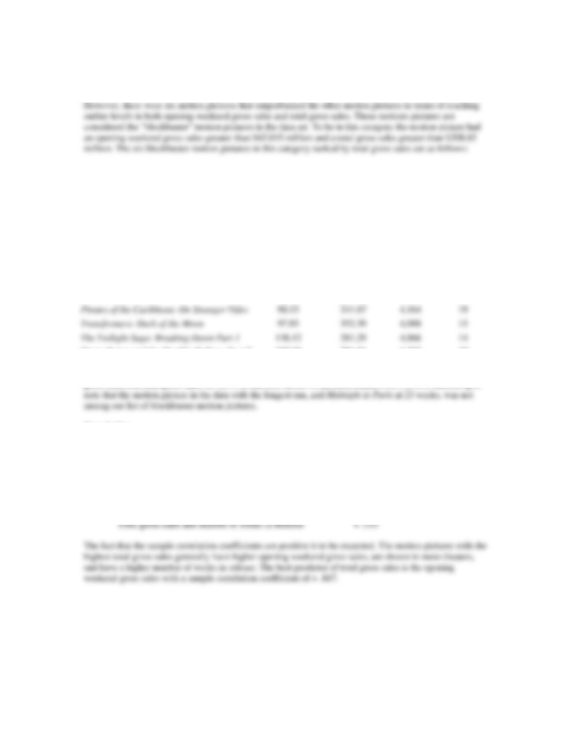
Pirates of the Caribbean: On Stranger Tides
90.15
241.07
4,164
19
Transformers: Dark of the Moon
97.85
352.39
4,088
15
The Twilight Saga: Breaking Dawn Part 1
138.12
281.29
4,066
14
Harry Potter and the Deathly Hallows Part 2
169.19
381.01
4,375
19
Harry Potter and the Deathly Hallows Part 2 was the top motion picture in terms of both opening weekend
gross sales and total gross sales for 2011. It was also shown in the most theaters (4375). It is interesting to
Correlation
We also computed the sample correlation coefficient between total gross sales and each of the other three
variables. Positive correlations were shown for all three relationships.
Total gross sales and opening weekend gross sales + .887
Total gross sales and number of theaters + .641
Case Problem 3: Heavenly Chocolates Website Traffic
1. Descriptive statistics for the time spent on the website, number of pages viewed, and amount spent
are shown below.
Time (min)
Pages Viewed
Amount Spent ($)
Mean
12.8
4.8
68.13
Median
11.4
4.5
62.15
Standard Deviation
6.06
2.04
32.34
Skewness
1.45
.65
1.05
Range
28.6
8
140.67
Minimum
4.3
2
17.84
Maximum
32.9
10
158.51
Sum
640.5
241
3406.41
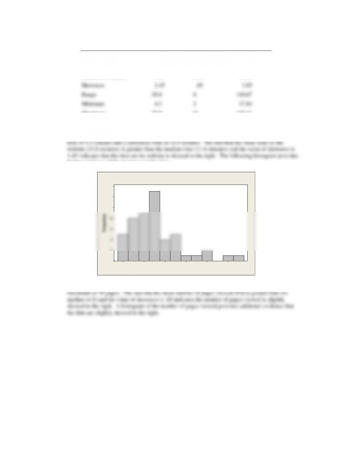
The mean time a shopper is on the Heavenly Chocolates website is 12.8 minutes, with a minimum
further evidence of the skewness in the data.
The mean number of pages viewed during a visit is 4.8 pages with a minimun of 2 pages and a
30252015105
14
12
10
8
6
4
2
0
Time (min)
Frequency
Histogram of Time (min)
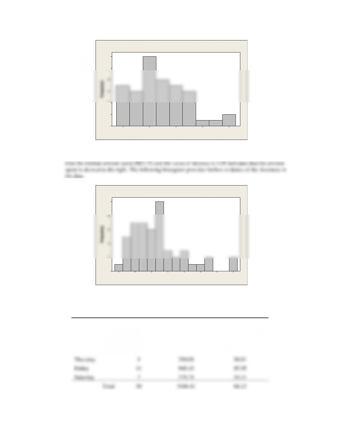
The mean amount spent for an on-line shopper is $68.13 with a minimum amount spent of $17.84
and a maximum amount spent of $158.51. The fact that the median amount spent ($68.13) is greater
2. Summary by Day of Week
Day of Week
Frequency
Total Amount
Spent ($)
Average Amount
Spent ($)
Sunday
5
218.15
43.63
Monday
9
813.38
90.38
Tuesday
7
414.86
59.27
Wednesday
6
341.82
56.97
Thursday
5
294.03
58.81
Friday
11
945.43
85.95
Saturday
7
378.74
54.11
50
68.13
108642
12
10
8
6
4
2
0
Pages Viewed
Frequency
Histogram of Pages Viewed
16014012010080604020
10
8
6
4
2
0
Amount
Frequency
Histogram of Amount
The above summary shows that Monday and Friday are the best days in terms of both the total
amount spent and the averge amount spent per transaction. Friday had the most purchases (11) and
the highest value for total amount spent ($945.43). Monday, with nine transactions, had the highest
3. Summary by Type of Browser
Browser
Frequency
Total Amount
Spent ($)
Average Amount
Spent ($)
Firefox
16
1228.21
76.76
Internet Explorer
27
1656.81
61.36
Other
7
521.39
74.48
Internet Explorer was used by 27 of the 50 shoppers (54%). But, the average amount spent spent by
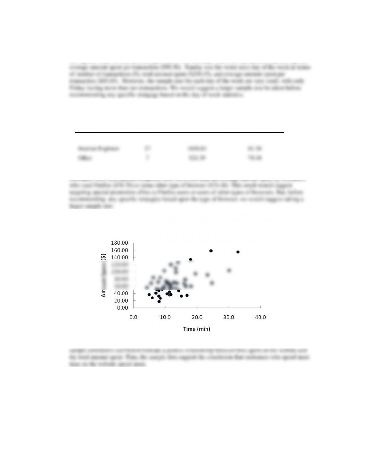
4. A scatter diagram showing the relationship between time spent on the website and the amount spent
follows:
The sample correlation coefficient between these two variables is .580. The scatter diagram and the
5. A scatter diagram showing the relationship between the number of pages viewed and the amount
spent follows:
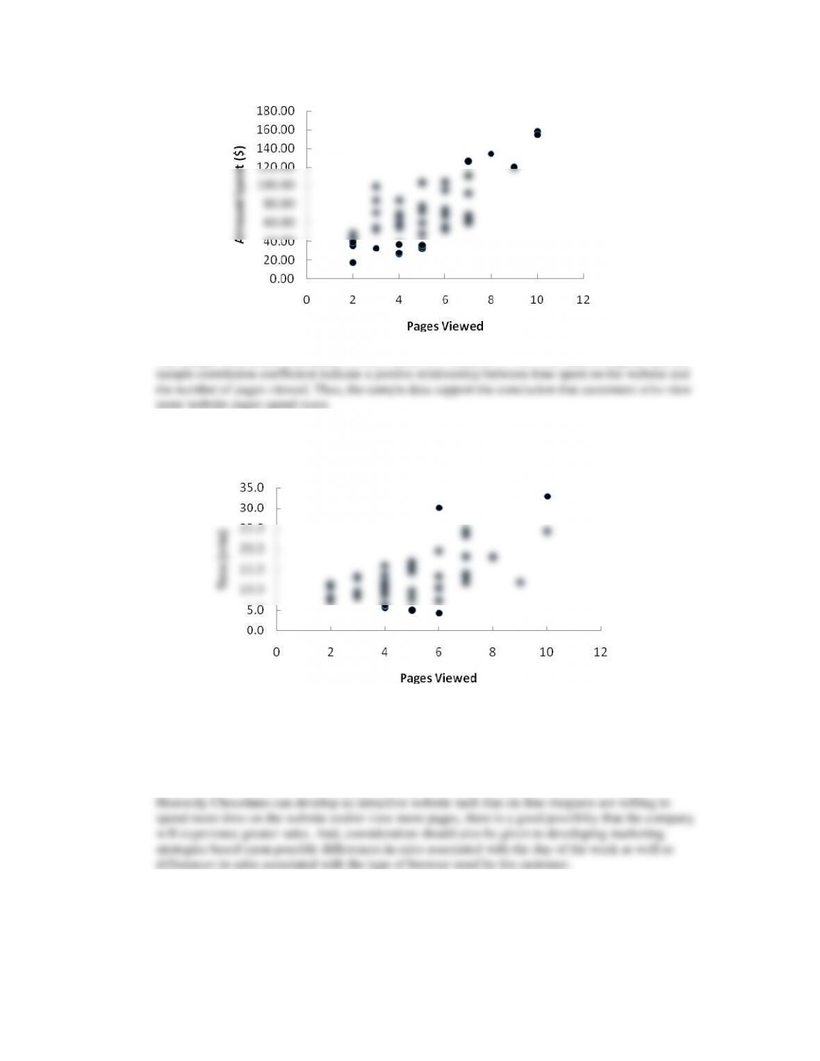
The sample correlation coefficient between these two variables is .724. The scatter diagram and the
6. A scatter diagram showing the relationship between the number of pages viewed and the time spent
on the website follows:
The sample correlation coefficient between these two variables is .596. The scatter diagram and the
sample correlation coefficient indicate a postive relationship between the number of pages viewed
and the time spent on the website.
Summary: The analysis indicates that on-line shoppers who spend more time on the company’s
website and/or view more website pages spend more money during their visit to the website. If
Case Problem 4: African Elephant Populations
This case provides the student with the opportunity to use the geometric mean in conjunction with a graph
(such as the boxplot) to analyze changes over time in the populations of elephants in several African
nations.
1. Let’s calculate the proportional change for each country over the ten year period 1979–1989. We’ll
begin by considering the Central African Republic. We have:
So the mean annual change in the elephant population for the Central African Republic during this
Repeating these calculations for each nation yields the values in the following table.
Country
( )( ) ( )
1 2 10
x x x
g
x
Mean Annual
Change
Angola
1.0000
1.0000
0.0000
Botswana
2.5500
1.0981
0.0981
Cameroon
1.3086
1.0273
0.0273
Cen African Rep
0.3016
0.8870
-0.1130
Chad
0.2067
0.8541
-0.1459
Congo
6.4815
1.2055
0.2055
Dem Rep of Congo
0.2250
0.8614
-0.1386
Gabon
5.6716
1.1895
0.1895
Kenya
0.2923
0.8843
-0.1157
Mozambique
0.3394
0.8976
-0.1024
Somalia
0.2469
0.8695
-0.1305
Sudan
0.0299
0.7039
-0.2961
Tanzania
0.2529
0.8716
-0.1284
Zambia
0.2733
0.8784
-0.1216
Zimbabwe
1.4333
1.0367
0.0367
The elephant populations in several nations (Central African Republic, Chad, Democratic Republic
of the Congo, Kenya, Mozambique, Somalia, Sudan, Tanzania, and Zambia) declined at an annual
2. Now let’s calculate the proportional change for each country over the ten year period 1989–2007.
We’ll again begin by considering the Central African Republic. We have:
3334=19000
( )( ) ( )
1 2 18
x x x
, so
( )( ) ( )
1 2 18
x x x
=0.175474 and
So the mean annual change in the elephant population for the Central African Republic during this
period is (0.907845 – 1)100 = –9.2155%. During the period of 1979-1989, the elephant population in
Country
( )( ) ( )
1 2 18
x x x
g
x
Mean Annual
Change
Angola
0.2040
0.9155
-0.0845
Botswana
3.4409
1.0711
0.0711
Cameroon
0.7258
0.9824
-0.0176
Cen African Rep
0.1755
0.9078
-0.0922
Chad
2.0758
1.0414
0.0414
Congo
0.3157
0.9380
-0.0620
Dem Rep of Congo
0.2790
0.9315
-0.0685
Gabon
0.9294
0.9959
-0.0041
Kenya
1.6651
1.0287
0.0287
Mozambique
1.4026
1.0190
0.0190
Somalia
0.0117
0.7809
-0.2191
Sudan
0.0750
0.8660
-0.1340
Tanzania
2.0875
1.0417
0.0417
Zambia
0.7130
0.9814
-0.0186
Zimbabwe
2.3048
1.0475
0.0475
Only two countries (Somalia and Sudan) continue to experience average annual declines in their
elephant populations of 10% or more from 1989-2007, while the elephant populations in most other
3. Now we compare the results of our two analyses and draw conclusions.
Country
Mean Annual Change
1979-1989
Mean Annual Change
1989-2007
Dem Rep of Congo
-0.1386
-0.0685
Tanzania
-0.1284
0.0417
Zambia
-0.1216
-0.0186
Sudan
-0.2961
-0.1340
Kenya
-0.1157
0.0287
Cen African Rep
-0.1130
-0.0922
Mozambique
-0.1024
0.0190
Zimbabwe
0.0367
0.0475
Somalia
-0.1305
-0.2191
Botswana
0.0981
0.0711
Cameroon
0.0273
-0.0176
Chad
-0.1459
0.0414
Gabon
0.1895
-0.0041
Angola
0.0000
-0.0845
Congo
0.2055
-0.0620
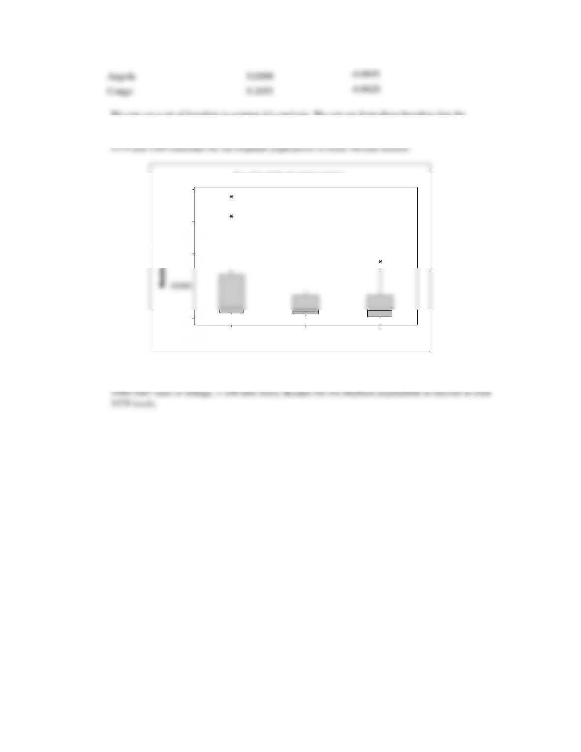
We can use a set of boxplots to support this analysis. We can see from these boxplots that the
population of elephants declined dramatically from 1979 to 1989, and have generally started to come
back between 1989 and 2007. We can also see that the declining trend that was established between
200719891979
400000
300000
200000
100000
0
Year
Elephant Population
Boxplot of Elephant Population
Several nations appear to have reversed the declines in elephant populations they experienced from
1979-1989, but the growth rates are still generally low (and in some countries still negative). At