Unlock document.
This document is partially blurred.
Unlock all pages and 1 million more documents.
Get Access
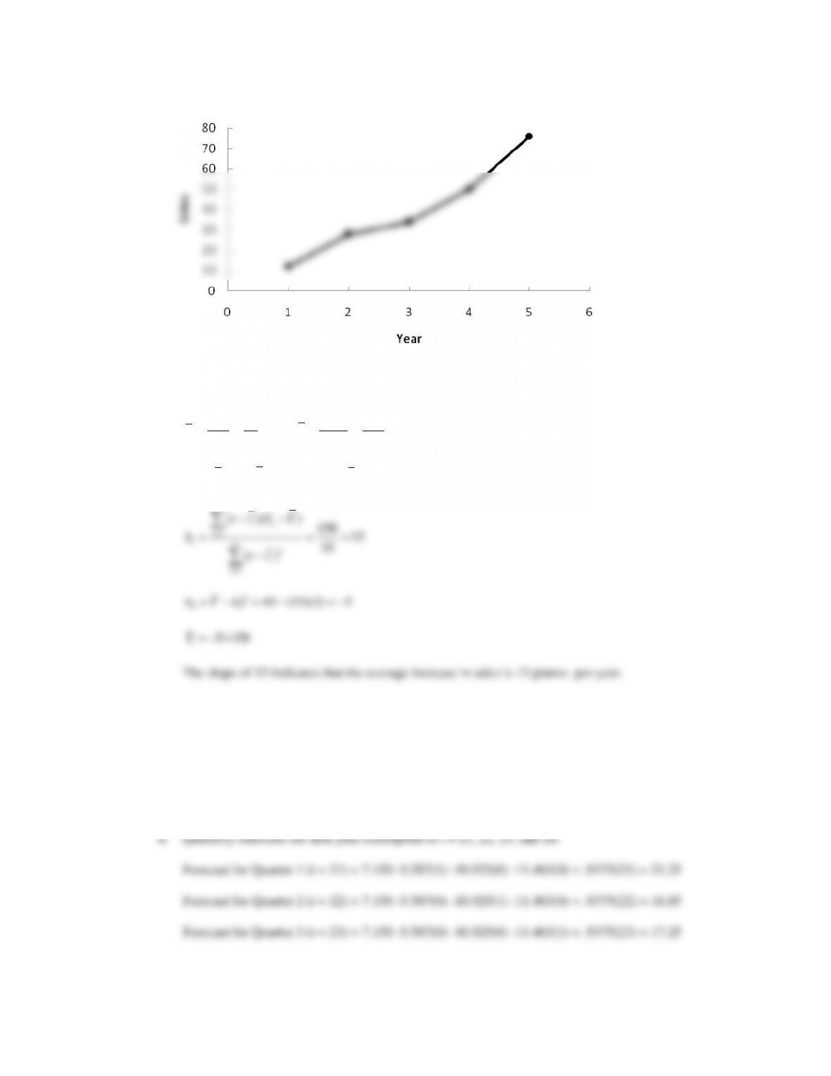
48. a.
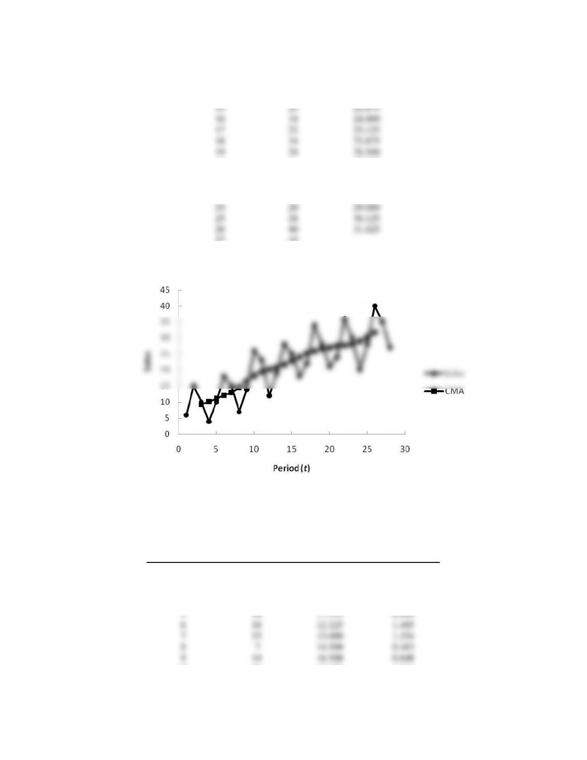
The time series plot shows a linear trend.
b.
11
15 200
3 40
55
nn
t
tt
tY
tY
nn
==
= = = = = =
2
( )( ) 150 ( ) 10
t
t t Y Y t t − − = − =
1
( )( ) 150 15
n
t
tn
t t Y Y
=
−−
t
Sales
Centered
Moving Average
Seasonal-Irregular
Value
1
4
2
2
3
1
3.250
0.308
4
5
3.750
1.333
5
6
4.375
1.371
6
4
5.875
0.681
7
4
7.500
0.533
8
14
7.875
1.778
9
10
7.875
1.270
10
3
8.250
0.364
11
5
8.750
0.571
12
16
9.750
1.641
13
12
10.750
1.116
14
9
11.750
0.766
15
7
13.250
0.528
16
22
14.125
1.558
17
18
15.000
1.200
18
10
17.375
0.576
19
13
20
35
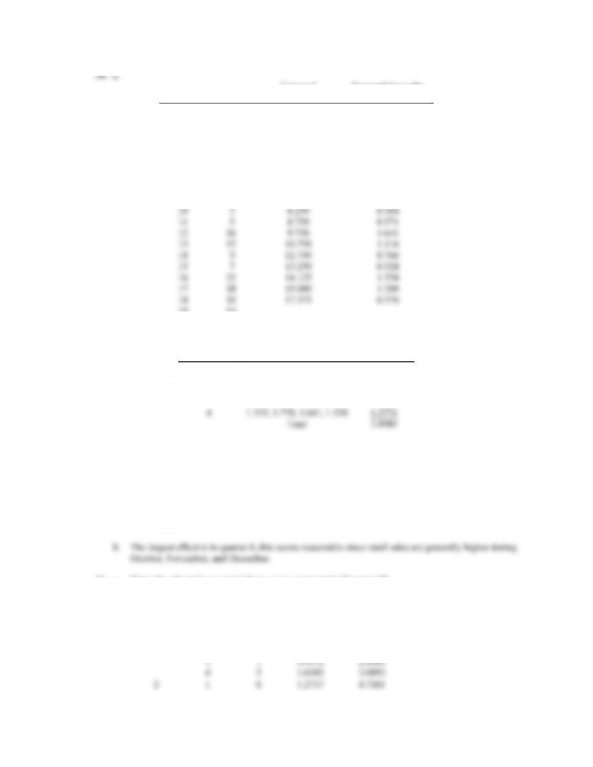
Quarter
Seasonal-Irregular
Values
Seasonal
Index
1
1.371, 1.270, 1.116, 1.200
1.2394
2
0.681, 0.364, 0.776, 0.576
0.5965
3
0.308, 0.533, 0.571, 0.528
0.4852
4
1.333, 1.778, 1.641, 1.558
1.5774
Total
3.8985
Quarter
Adjusted Seasonal Index
1
1.2717
2
0.6120
3
0.4978
4
1.6185
Note: Adjustment for seasonal index = 4 / 3.8985 = 1.0260
Year
Quarter
Sales
Adjusted
Seasonal
Index
Deseasonalized
Sales
1
1
4
1.2717
3.1454
2
2
0.6120
3.2680
3
1
0.4978
2.0088
4
5
1.6185
3.0893
2
1
6
1.2717
4.7181
2
4
0.6120
6.5359
3
4
0.4978
8.0354
4
14
1.6185
8.6500
3
1
10
1.2717
7.8635
2
3
0.6120
4.9020
3
5
0.4978
10.0442
4
16
1.6185
9.8857
4
1
12
1.2717
9.4362
2
9
0.6120
14.7059
3
7
0.4978
14.0619
4
22
1.6185
13.5928
5
1
18
1.2717
14.1543
2
10
0.6120
16.3399
3
13
0.4978
26.1149
4
35
1.6185
21.6250
Using Excel’s Regression tool, the estimated regression equation is:
Deseasonalized Sales = - 0.36 + 0.997t
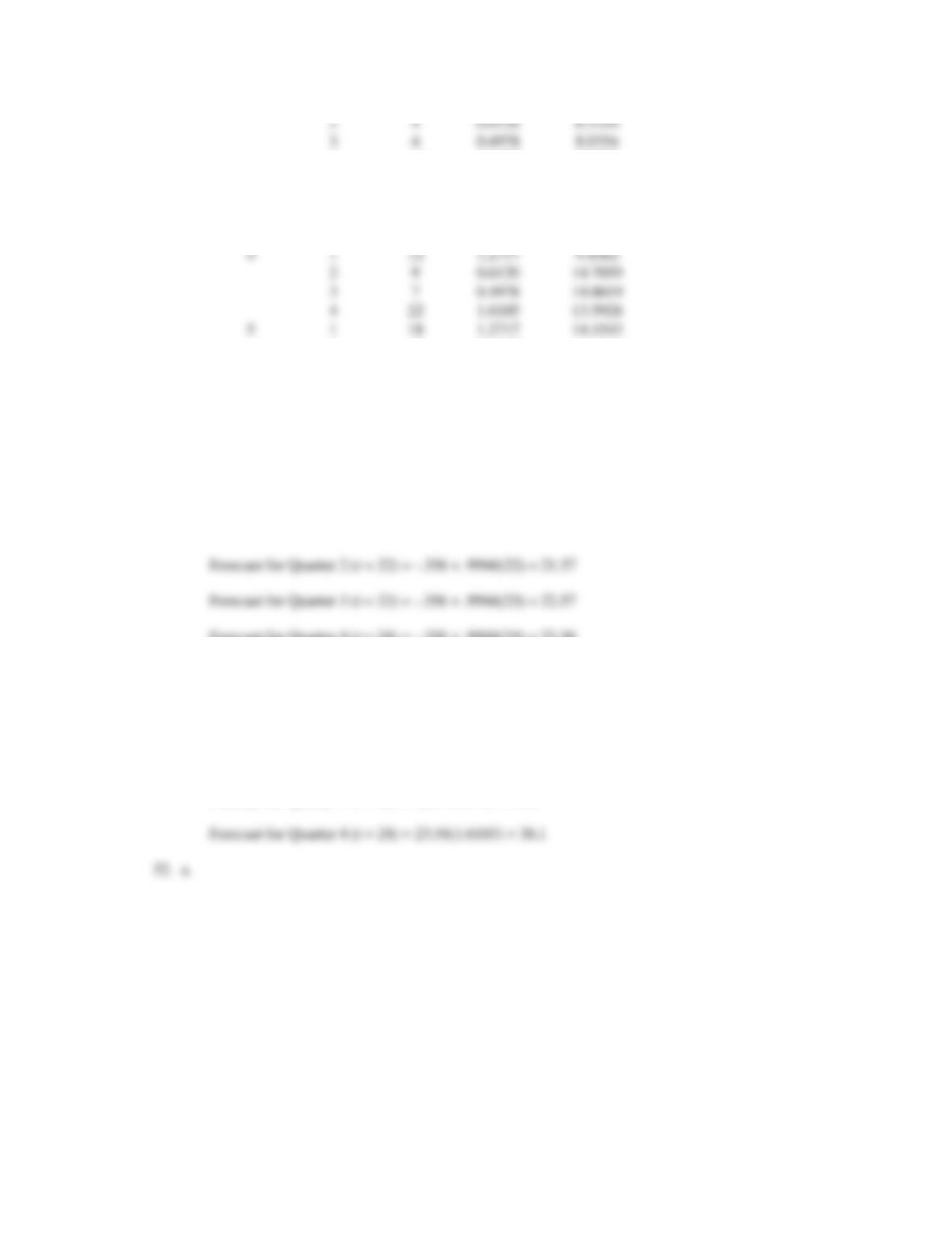
b. The quarterly trend forecasts for next year correspond to t = 21, 22, 23, and 24.
Forecast for Quarter 1 (t = 21) = -.356 + .9966(21) = 20.57
Forecast for Quarter 4 (t = 24) = -.356 + .9966(24) = 23.56
c. Multiplying the quarterly trend forecasts by the adjusted seasonal indexes provides the forecasts for
next year.
Forecast for Quarter 1 (t = 21) = 20.57(1.2717) = 26.2
Forecast for Quarter 2 (t = 22) = 21.57(.6120) = 13. 2
Forecast for Quarter 3 (t = 23) = 22.57(.4978) = 11.2
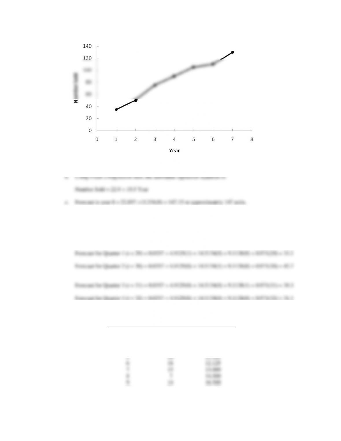
A linear trend pattern appears to be present in the time series plot.
53. a. Using Excel’s Regression tool, the estimated multiple regression equation is:
Sales = 0.036 + 4.91 Qtr1 + 14.5 Qtr2 + 9.11 Qtr3 + 0.971t
b. The quarterly forecast for next year correspond to t = 29, 30, 31, and 32.
54. a.
t
Sales
Centered
Moving Average
1
6
2
15
3
10
9.250
4
4
10.125
5
10
11.125
6
18
12.125
7
15
13.000
8
7
14.500
9
14
16.500
10
26
18.125
11
23
19.375
12
12
20.250
13
19
20.750
14
28
21.750
15
25
22.875
16
18
24.000
17
22
25.125
18
34
25.875
19
28
26.500
20
21
27.000
21
24
27.500
22
36
27.625
23
30
28.000
24
20
29.000
25
28
30.125
26
40
31.625
27
35
28
27
b.
The centered moving average values smooth out the time series by removing seasonal effects and
some of the random variability. The centered moving average time series shows the trend in the data.
c.
t
Sales
Centered
Moving Average
Seasonal-Irregular
Value
1
6
2
15
3
10
9.250
1.081
4
4
10.125
0.395
5
10
11.125
0.899
6
18
12.125
1.485
7
15
13.000
1.154
8
7
14.500
0.483
9
14
16.500
0.848
10
26
18.125
1.434
11
23
19.375
1.187
12
12
20.250
0.593
13
19
20.750
0.916
14
28
21.750
1.287
15
25
22.875
1.093
16
18
24.000
0.750
17
22
25.125
0.876
18
34
25.875
1.314
19
28
26.500
1.057
20
21
27.000
0.778
21
24
27.500
0.873
22
36
27.625
1.303
23
30
28.000
1.071
24
20
29.000
0.690
25
28
30.125
0.929
26
40
31.625
1.265
27
35
28
27
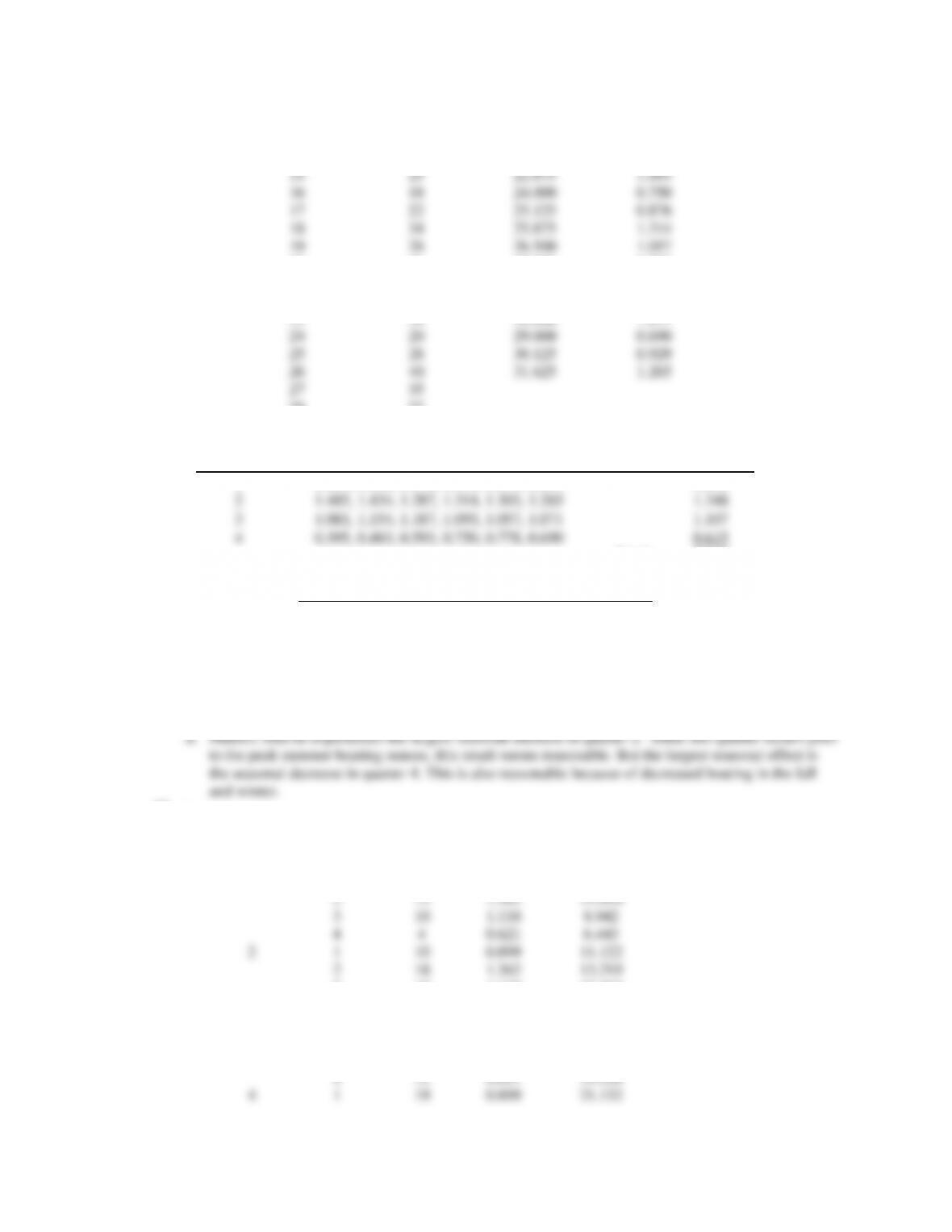
Quarter
Seasonal-Irregular
Component Values
Seasonal
Index
1
0.899, 0.848, 0.916, 0.876, 0.873, 0.929
0.890
2
1.485, 1.434, 1.287, 1.314, 1.303, 1.265
1.348
3
1.081, 1.154, 1.187, 1.093, 1.057, 1.071
1.107
4
0.395, 0.483, 0.593, 0.750, 0.778, 0.690
0.615
Total
3.960
Quarter
Adjusted Seasonal Index
1
0.899
2
1.362
3
1.118
4
0.621
Note: Adjustment for seasonal index = 4.00 / 3.96 = 1.0101
55. a.
Year
Quarter
Sales
Adjusted
Seasonal
Index
Deseasonalized
Sales
1
1
6
0.899
6.673
2
15
1.362
11.016
3
10
1.118
8.942
4
4
0.621
6.443
2
1
10
0.899
11.122
2
18
1.362
13.219
3
15
1.118
13.413
4
7
0.621
11.275
3
1
14
0.899
15.571
2
26
1.362
19.094
3
23
1.118
20.566
4
12
0.621
19.328
4
1
19
0.899
21.132
2
28
1.362
20.563
3
25
1.118
22.355
4
18
0.621
28.993
5
1
22
0.899
24.468
2
34
1.362
24.969
3
28
1.118
25.037
4
21
0.621
33.825
6
1
24
0.899
26.692
2
36
1.362
26.438
3
30
1.118
26.825
4
20
0.621
32.214
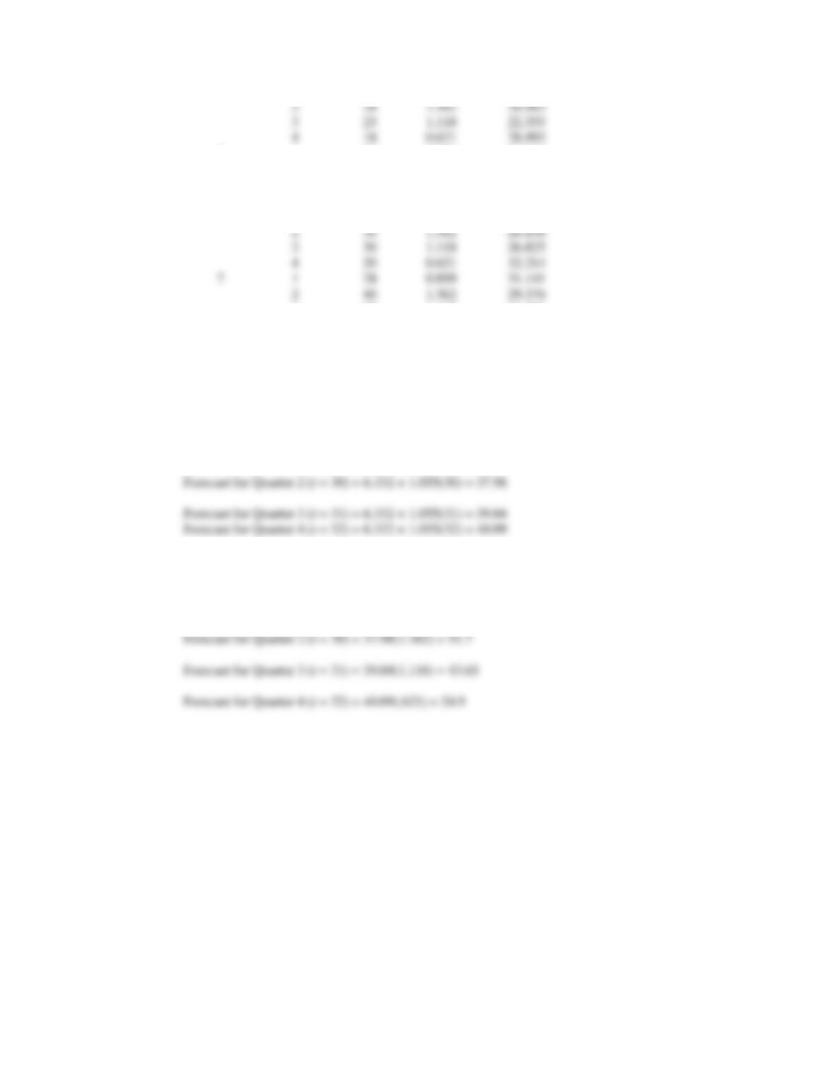
7
1
28
0.899
31.141
2
40
1.362
29.376
3
35
1.118
31.296
4
27
0.621
43.489
Using Excel’s Regression tool, the estimated multiple regression equation is:
Deseasonalized Sales = 6.33 + 1.05t
b. The quarterly forecast for next year correspond to t = 29, 30, 31, and 32.
Forecast for Quarter 1 (t = 29) = 6.332 + 1.055(29) = 36.93
c. Multiplying the quarterly trend forecasts by the adjusted seasonal indexes provides the forecasts for
next year.
Forecast for Quarter 1 (t = 29) = 36.93(.899) = 33.2


