Unlock document.
This document is partially blurred.
Unlock all pages and 1 million more documents.
Get Access
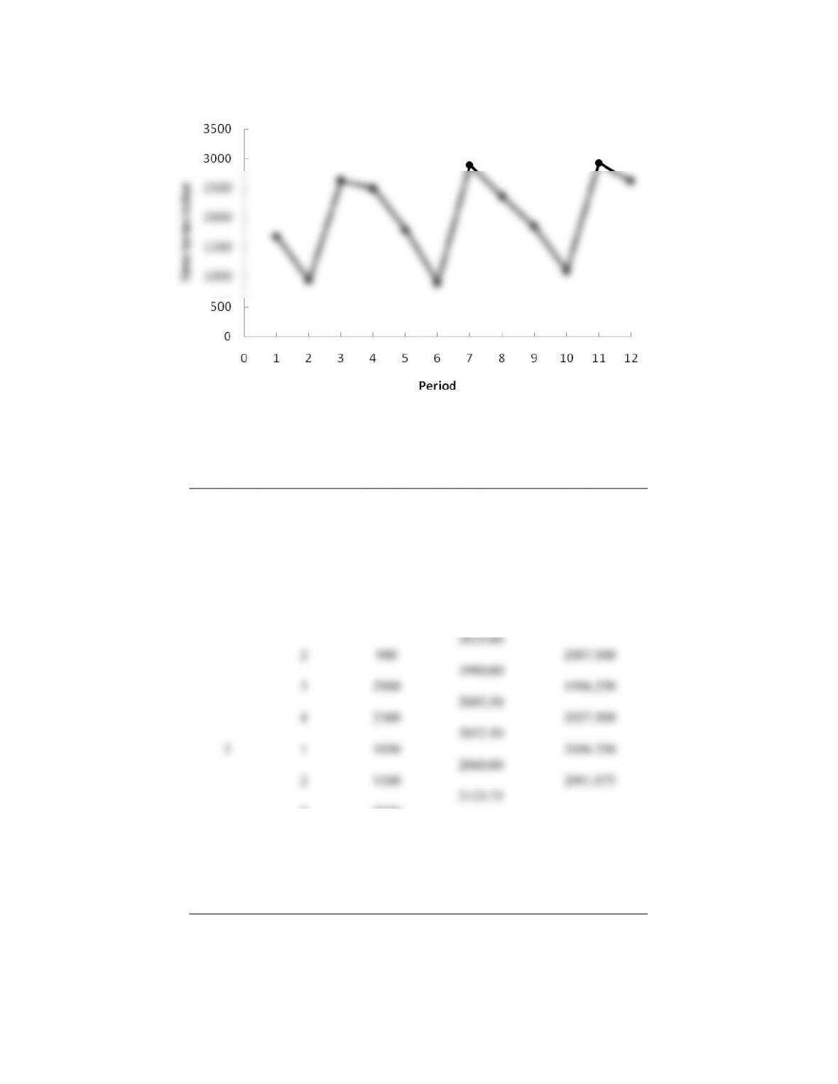
37. a.
The time series plot indicates linear trend and seasonal pattern.
b.
Year
Quarter
Time Series
Value
Four-Quarter
Moving Average
Centered Moving
Average
1
1
1690
2
940
1938.75
3
2625
1952.500
1966.25
4
2500
1961.250
1956.25
2
1
1800
1990.625
2025.00
2
900
2007.500
1990.00
3
2900
1996.250
2002.50
4
2360
2027.500
2052.50
3
1
1850
2056.250
2060.00
2
1100
2091.875
2123.75
3
2930
4
2615
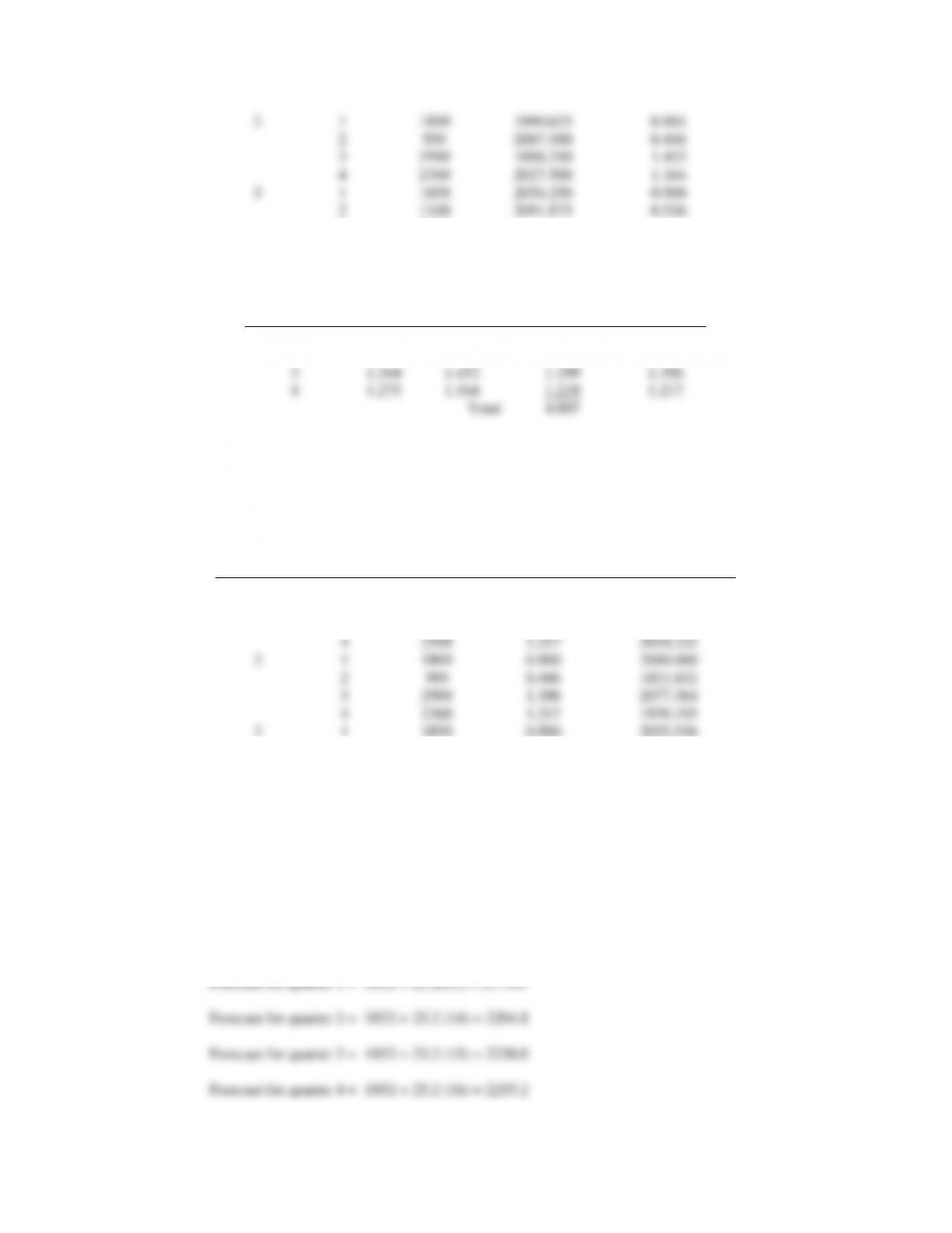
c.
Year
Quarter
Time Series
Value
Centered Moving
Average
Seasonal-Irregular
Value
1
1
1690
2
940
3
2625
1952.500
1.344
4
2500
1961.250
1.275
2
1
1800
1990.625
0.904
2
900
2007.500
0.448
3
2900
1996.250
1.453
4
2360
2027.500
1.164
3
1
1850
2056.250
0.900
2
1100
2091.875
0.526
3
2930
4
2615
Quarter
Seasonal-Irregular
Values
Seasonal Index
Adjusted
Seasonal
Index
1
0.904
0.900
0.902
0.900
2
0.448
0.526
0.487
0.486
3
1.344
1.453
1.399
1.396
4
1.275
1.164
1.219
1.217
Total
4.007
Note: Adjustment for seasonal index = 4.000 / 4.007 = 0.998
d. The largest school effect is in the third quarter which corresponds to back-to-school demand during
July, August, and September of each year.
e.
Year
Quarter
Time Series
Value
Adjusted
Seasonal Index
Deseasonalized
Value
1
1
1690
0.900
1877.778
2
940
0.486
1934.156
3
2625
1.396
1880.372
4
2500
1.217
2054.232
2
1
1800
0.900
2000.000
2
900
0.486
1851.852
3
2900
1.396
2077.364
4
2360
1.217
1939.195
3
1
1850
0.900
2055.556
2
1100
0.486
2263.374
3
2930
1.396
2098.854
4
2615
1.217
2148.726
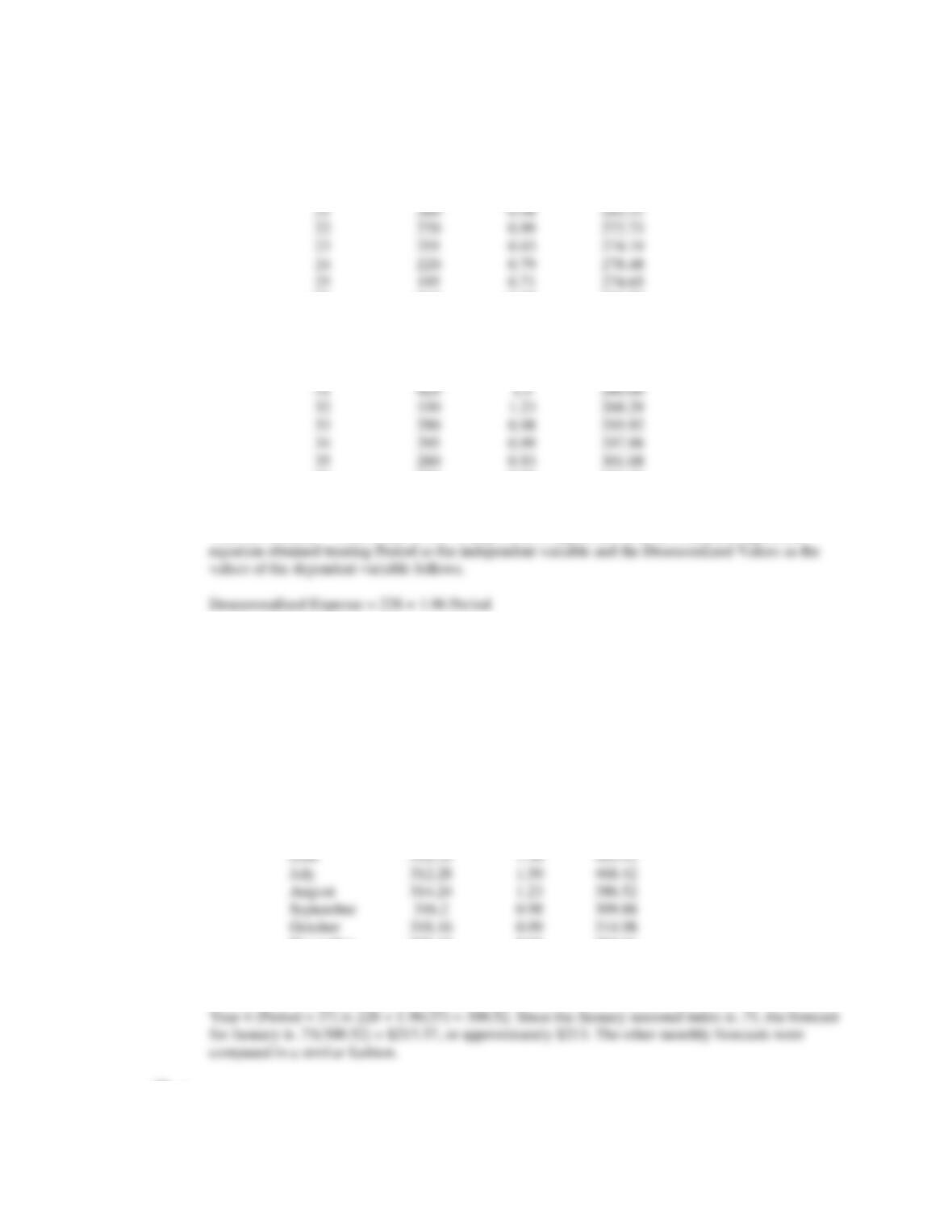
f. Let Period = 1 denote the time series value in Year 1 – Quarter 1; Period = 2 denote the time series
value in Year 1 – Quarter 2; and so on. Using Excel’s Regression tool, the estimated regression
equation obtained treating Period as the independent variable and the Deseasonlized Values as the
values of the dependent variable follows.
Deseasonalized Value = 1852 + 25.2 Period
The quarterly deseasonalized trend forecasts for Year 4 (Periods 13, 14, 15, and 16) are as follows:
g. Adjusting the quarterly deseasonalized trend forecasts provides the following quarterly estimates:
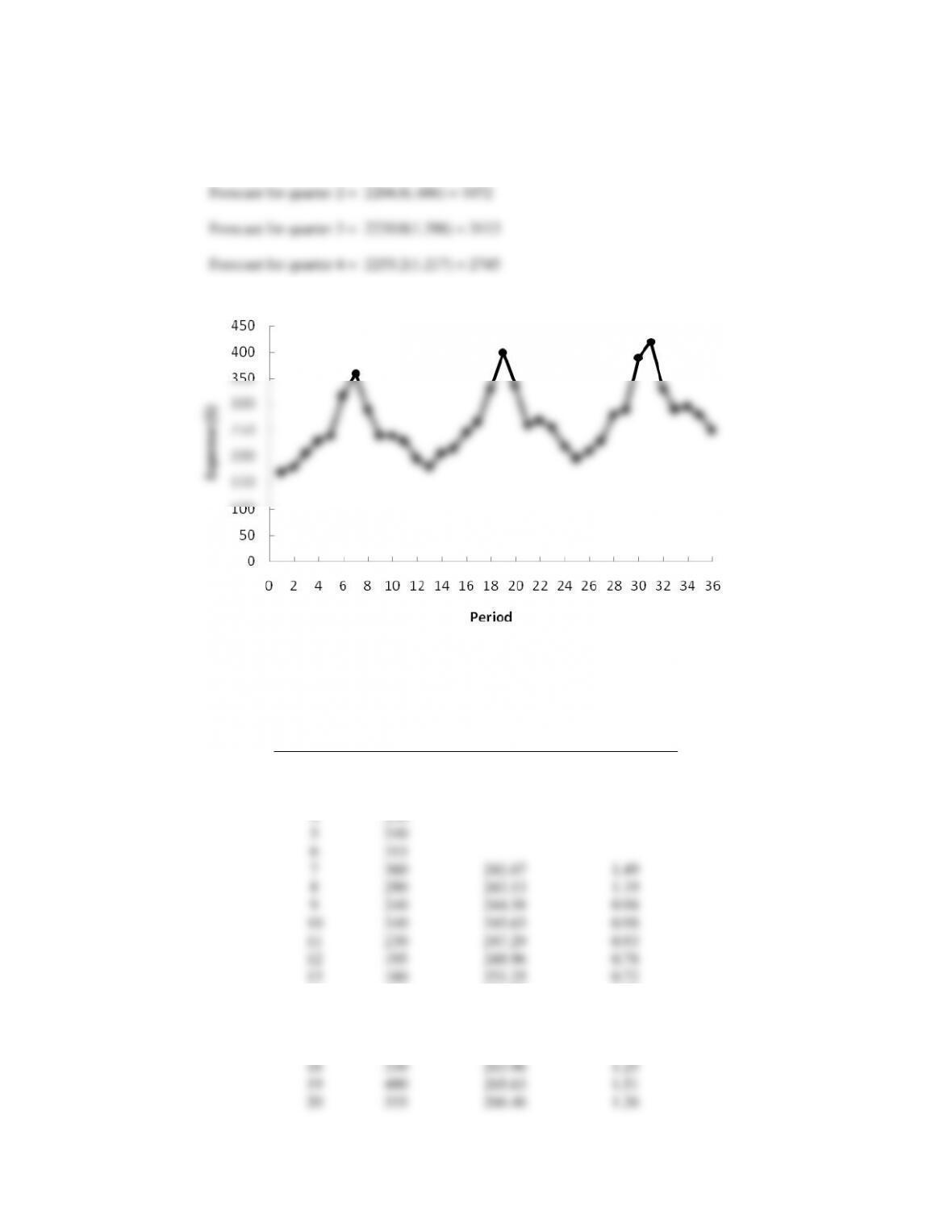
Forecast for quarter 1 = 2179.6(.900) = 1962
38. a.
The time series plot shows a linear trend and seasonal effects.
b.
Month
Expense
Centered Moving
Average
Seasonal-
Irregular
Value
1
170
2
180
3
205
4
230
5
240
6
315
7
360
241.67
1.49
8
290
243.13
1.19
9
240
244.58
0.98
10
240
245.63
0.98
11
230
247.29
0.93
12
195
248.96
0.78
13
180
251.25
0.72
14
205
254.79
0.80
15
215
257.50
0.83
16
245
259.58
0.94
17
265
261.88
1.01
18
330
263.96
1.25
19
400
265.63
1.51
20
335
266.46
1.26
21
260
267.29
0.97
22
270
269.38
1.00
23
255
271.88
0.94
24
220
275.42
0.80
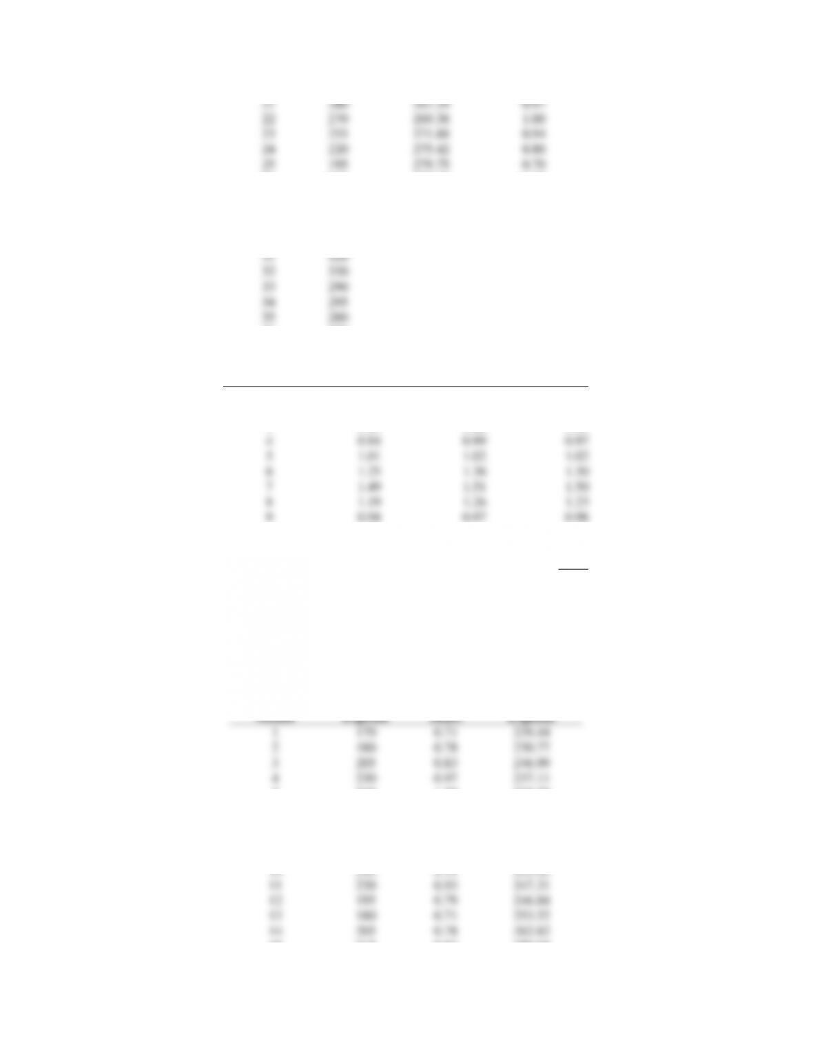
25
195
278.75
0.70
26
210
279.38
0.75
27
230
280.42
0.82
28
280
282.71
0.99
29
290
284.79
1.02
30
390
287.08
1.36
31
420
32
330
33
290
34
295
35
280
36
250
Month
Seasonal-Irregular
Values
Seasonal
Index
1
0.72
0.70
0.71
2
0.80
0.75
0.78
3
0.83
0.82
0.83
4
0.94
0.99
0.97
5
1.01
1.02
1.02
6
1.25
1.36
1.30
7
1.49
1.51
1.50
8
1.19
1.26
1.23
9
0.98
0.97
0.98
10
0.98
1.00
0.99
11
0.93
0.94
0.93
12
0.78
0.80
0.79
Total
12.03
Notes: 1. Adjustment for seasonal index = 12 / 12.03 = 0.998
2. Because the seasonal-irregular values and the seasonal index values were rounded
to two decimal places to simplify the presentation, the adjustment is really not
necessary in this problem since it implies more accuracy than is warranted.
c.
Month
Expense
Seasonal
Index
Deseasonalized
Expense
1
170
0.71
239.44
2
180
0.78
230.77
3
205
0.83
246.99
4
230
0.97
237.11
5
240
1.02
235.29
6
315
1.3
242.31
7
360
1.5
240.00
8
290
1.23
235.77
9
240
0.98
244.90
10
240
0.99
242.42
11
230
0.93
247.31
12
195
0.79
246.84
13
180
0.71
253.52
14
205
0.78
262.82
15
215
0.83
259.04
16
245
0.97
252.58
17
265
1.02
259.80
18
330
1.3
253.85
19
400
1.5
266.67
20
335
1.23
272.36
21
260
0.98
265.31
22
270
0.99
272.73
23
255
0.93
274.19
24
220
0.79
278.48
25
195
0.71
274.65
26
210
0.78
269.23
27
230
0.83
277.11
28
280
0.97
288.66
29
290
1.02
284.31
30
390
1.3
300.00
31
420
1.5
280.00
32
330
1.23
268.29
33
290
0.98
295.92
34
295
0.99
297.98
35
280
0.93
301.08
36
250
0.79
316.46
d. Let Period = 1 denote the time series value in January – Year 1; Period = 2 denote the time series
value in February – Year 2; and so on. Using Excel’s Regression tool, the estimated regression
e. The linear trend estimates for the deseasonalized time series and the adjustment based upon the
seasonal effects are shown below.
Month
Deseasonalized
Trend Forecast
Seasonal
Index
Monthly
Forecast
January
300.52
0.71
213.37
February
302.48
0.78
235.93
March
304.44
0.83
252.69
April
306.4
0.97
297.21
May
308.36
1.02
314.53
June
310.32
1.30
403.42
July
312.28
1.50
468.42
August
314.24
1.23
386.52
September
316.2
0.98
309.88
October
318.16
0.99
314.98
November
320.12
0.93
297.71
December
322.08
0.79
254.44
For instance, using the estimated regression equation the deseasonalized trend forecast for January in
39. a.
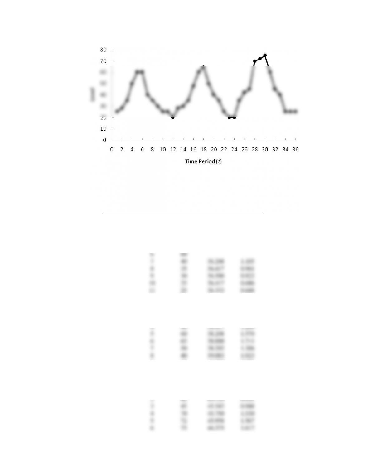
The time series plot indicates a seasonal pattern in the data and perhaps a slight upward linear trend.
b.
Day
Hour
Reading
Centered
Moving
Average
Seasonal-
Irregular
Value
July 15
1
25
2
28
3
35
4
50
5
60
6
60
7
40
36.208
1.105
8
35
36.417
0.961
9
30
36.500
0.822
10
25
36.417
0.686
11
25
36.333
0.688
12
20
36.542
0.547
July 16
1
28
37.167
0.753
2
30
37.792
0.794
3
35
38.208
0.916
4
48
38.417
1.249
5
60
38.208
1.570
6
65
38.000
1.711
7
50
38.292
1.306
8
40
39.083
1.023
9
35
40.000
0.875
10
25
41.333
0.605
11
20
42.750
0.468
12
20
43.667
0.458
July 17
1
35
44.500
0.787
2
42
45.125
0.931
3
45
45.542
0.988
4
70
45.750
1.530
5
72
45.958
1.567
6
75
46.375
1.617
7
60
8
45
9
40
10
25
11
25
12
25
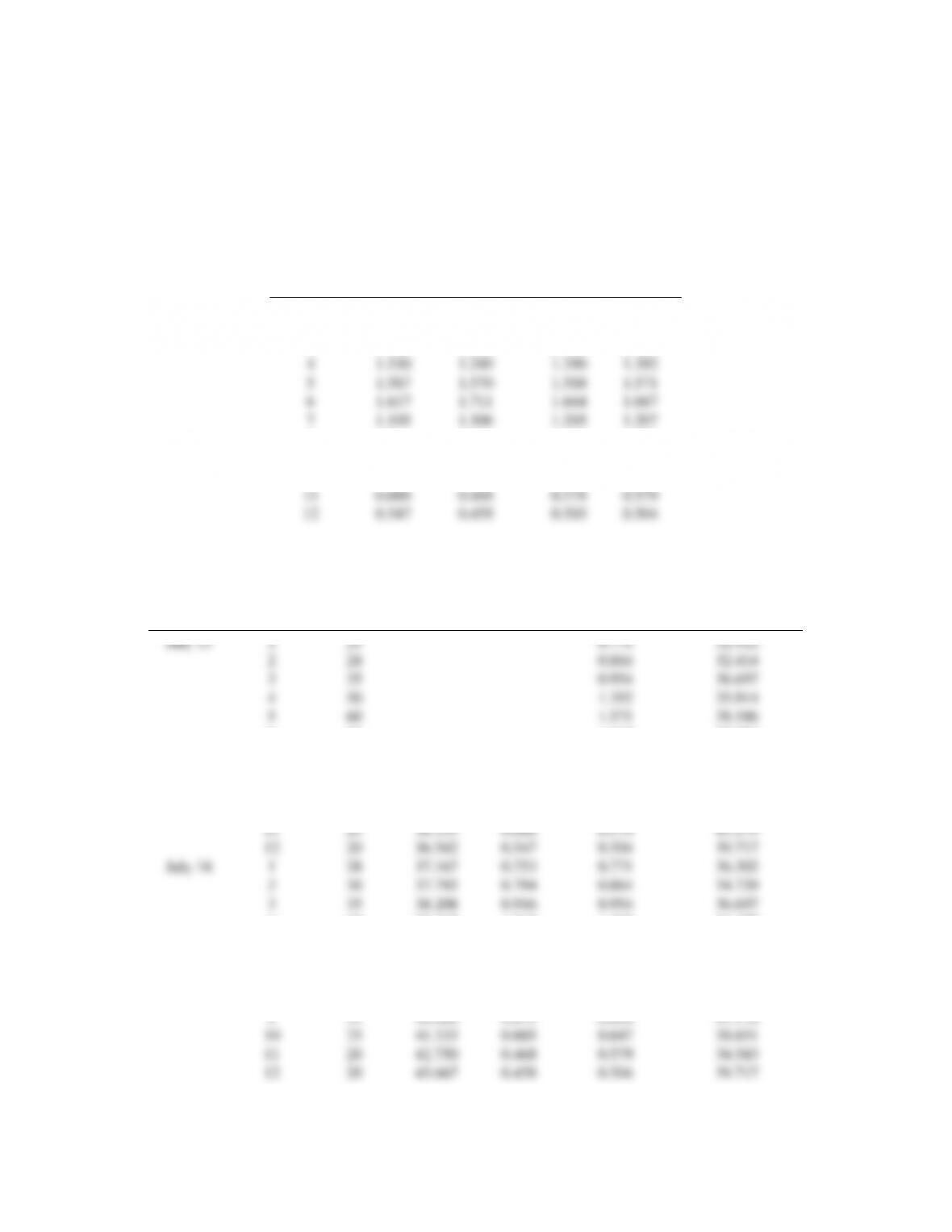
Hour
Seasonal-Irregular
Values
Seasonal
Index
Adjusted
Seasonal
Index
1
0.787
0.753
0.770
0.771
2
0.931
0.794
0.862
0.864
3
0.988
0.916
0.952
0.954
4
1.530
1.249
1.390
1.392
5
1.567
1.570
1.568
1.571
6
1.617
1.711
1.664
1.667
7
1.105
1.306
1.205
1.207
8
0.961
1.023
0.992
0.994
9
0.822
0.875
0.848
0.850
10
0.686
0.605
0.646
0.647
11
0.688
0.468
0.578
0.579
12
0.547
0.458
0.503
0.504
c. The adjusted seasonal indexes can now be used to deseasonalize the data as shown below.
Day
Hour
Reading
Centered
Moving
Average
Seasonal-
Irregular
Value
Seasonal Index
Deseasonalized
Reading
July 15
1
25
0.771
32.412
2
28
0.864
32.414
3
35
0.954
36.697
4
50
1.392
35.914
5
60
1.571
38.186
6
60
1.667
35.996
7
40
36.208
1.105
1.207
33.129
8
35
36.417
0.961
0.994
35.210
9
30
36.500
0.822
0.850
35.295
10
25
36.417
0.686
0.647
38.651
11
25
36.333
0.688
0.579
43.179
12
20
36.542
0.547
0.504
39.717
July 16
1
28
37.167
0.753
0.771
36.302
2
30
37.792
0.794
0.864
34.729
3
35
38.208
0.916
0.954
36.697
4
48
38.417
1.249
1.392
34.477
5
60
38.208
1.570
1.571
38.186
6
65
38.000
1.711
1.667
38.996
7
50
38.292
1.306
1.207
41.412
8
40
39.083
1.023
0.994
40.240
9
35
40.000
0.875
0.850
41.178
10
25
41.333
0.605
0.647
38.651
11
20
42.750
0.468
0.579
34.543
12
20
43.667
0.458
0.504
39.717
July 17
1
35
44.500
0.787
0.771
45.377
2
42
45.125
0.931
0.864
48.621
3
45
45.542
0.988
0.954
47.182
4
70
45.750
1.530
1.392
50.279
5
72
45.958
1.567
1.571
45.823
6
75
46.375
1.617
1.667
44.995
7
60
1.207
49.694
8
45
0.994
45.270
9
40
0.850
47.061
10
25
0.647
38.651
11
25
0.579
43.179
12
25
0.504
49.646
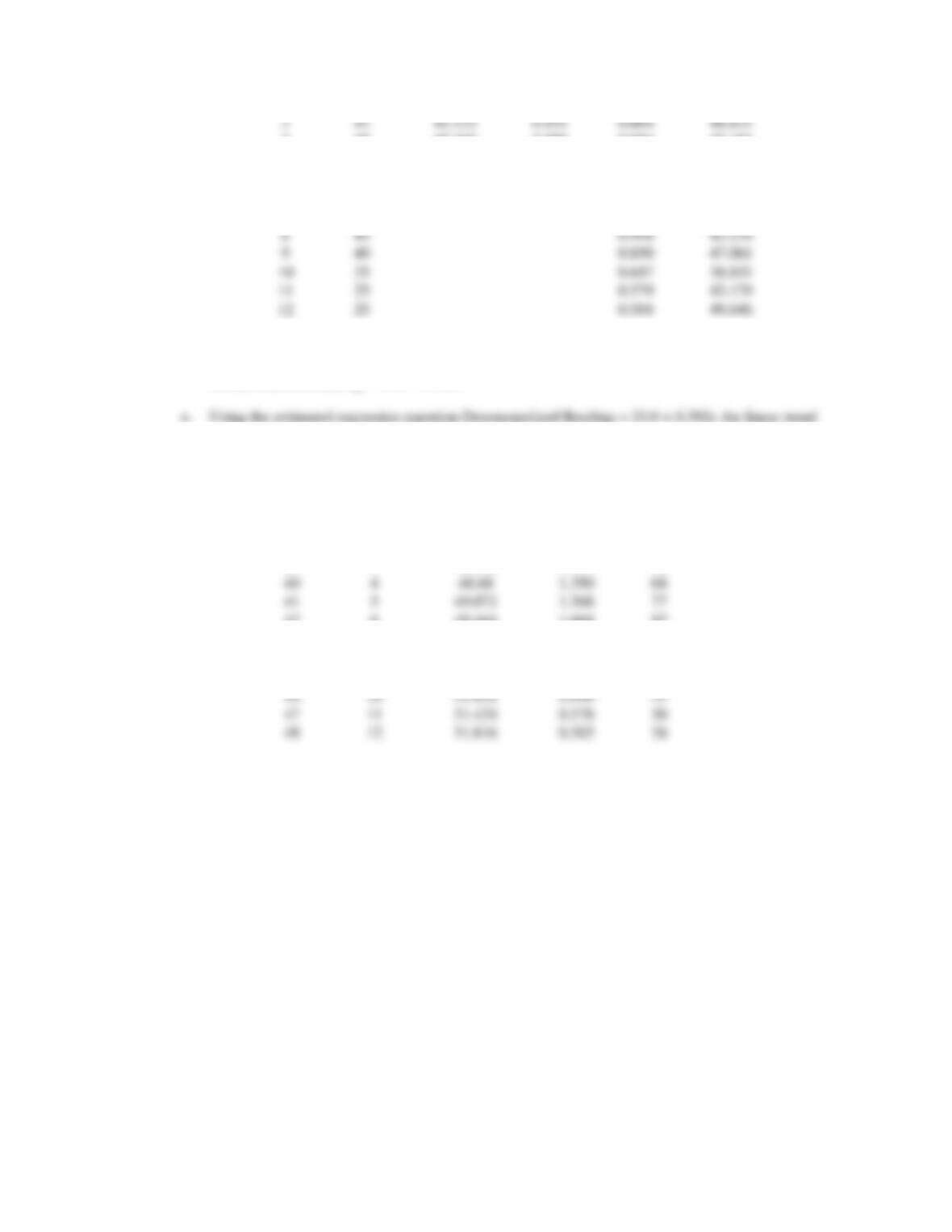
d. Using Excel’s Regression tool, the trend line fitted to the deseasonalized data is:
Deseasonalized Reading = 33.0 + 0.392t
estimates for the deseasonalized time series and the adjustment based upon the hourly effects are
shown below.
t
Hour
Deseasonalized
Trend Forecast
Seasonal
Index
Hourly
Forecast
37
1
47.504
0.770
37
38
2
47.896
0.862
41
39
3
48.288
0.952
46
40
4
48.68
1.390
68
41
5
49.072
1.568
77
42
6
49.464
1.664
82
43
7
49.856
1.205
60
44
8
50.248
0.992
50
45
9
50.64
0.848
43
46
10
51.032
0.646
33
47
11
51.424
0.578
30
48
12
51.816
0.503
26


