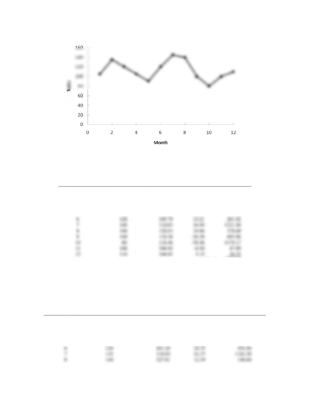
14. a.
The data appear to follow a horizontal pattern.
b. Smoothing constant = .3.
Month t
Time-Series Value
Yt
Forecast Ft
Forecast Error
Yt – Ft
Squared Error
(Yt – Ft)2
1
105
2
135
105.00
30.00
900.00
3
120
114.00
6.00
36.00
4
105
115.80
-10.80
116.64
5
90
112.56
-22.56
508.95
6
120
105.79
14.21
201.92
7
145
110.05
34.95
1221.50
8
140
120.54
19.46
378.69
9
100
126.38
-26.38
695.90
10
80
118.46
-38.46
1479.17
11
100
106.92
-6.92
47.89
12
110
104.85
5.15
26.52
Total
5613.18
MSE = 5613.18 / 11 = 510.29
Forecast for month 13: F13 = .3(110) + .7(104.85) = 106.4
c. Smoothing constant = .5
Month t
Time-Series Value
Yt
Forecast Ft
Forecast Error
Yt – Ft
Squared Error
(Yt – Ft)2
1
105
2
135
105
30.00
900.00
3
120
120
0.00
0.00
4
105
120
-15.00
225.00
5
90
112.50
-22.50
506.25
6
120
101.25
18.75
351.56
7
145
110.63
34.37
1181.30
8
140
127.81
12.19
148.60
9
100
133.91
-33.91
1149.89
10
80
116.95
-36.95
1365.30
11
100
98.48
1.52
2.31
12
110
99.24
10.76
115.78
5945.99
MSE = 5945.99 / 11 = 540.55
Forecast for month 13: F13 = .5(110) + .5(99.24) = 104.62
Conclusion: a smoothing constant of .3 is better than a smoothing constant of .5 since the MSE is less for 0.3.
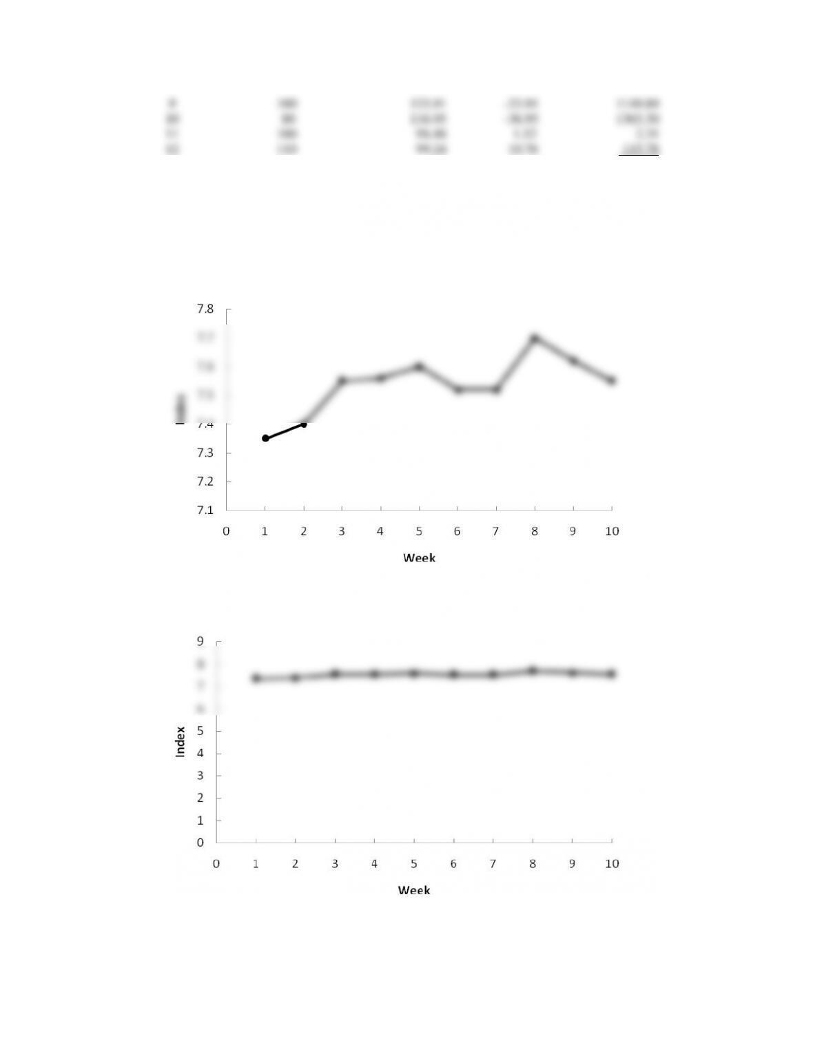
15. a.
You might think the time series plot shown above exhibits some trend. But, this is simply due to the
fact that the smallest value on the vertical axis is 7.1, as shown by the following version of the plot.
In other words, the time series plot shows an underlying horizontal pattern.
b/c.
Week
Time-Series
Value
α = .2
Forecast
(Error)2
α = .3
Forecast
(Error)2
1
7.35
2
7.40
7.35
.0025
7.35
.0025
3
7.55
7.36
.0361
7.36
.0361
4
7.56
7.40
.0256
7.42
.0196
5
7.60
7.43
.0289
7.46
.0196
6
7.52
7.46
.0036
7.50
.0004
7
7.52
7.48
.0016
7.51
.0001
8
7.70
7.48
.0484
7.51
.0361
9
7.62
7.53
.0081
7.57
.0025
10
7.55
7.55
.0000
7.58
.0009
.1548
.1178
d. MSE(α = .2) = .1548 / 9 = .0172
MSE(α = .3) = .1178 / 9 = .0131
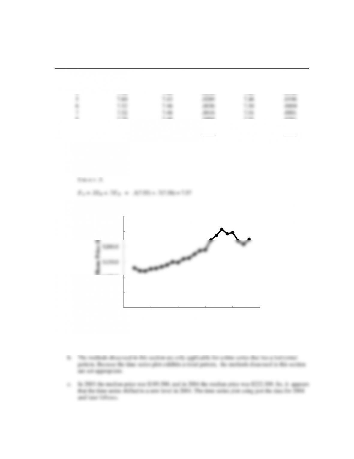
16. a.
The time series plot exhibits a trend pattern. Although the recession of 2008 led to a downturn in
prices, the median price rose form 2010 to 2011.
$0.0
$50.0
$100.0
$150.0
$200.0
$250.0
$300.0
1988 1993 1998 2003 2008 2013
Median Home Price ($000)
Year
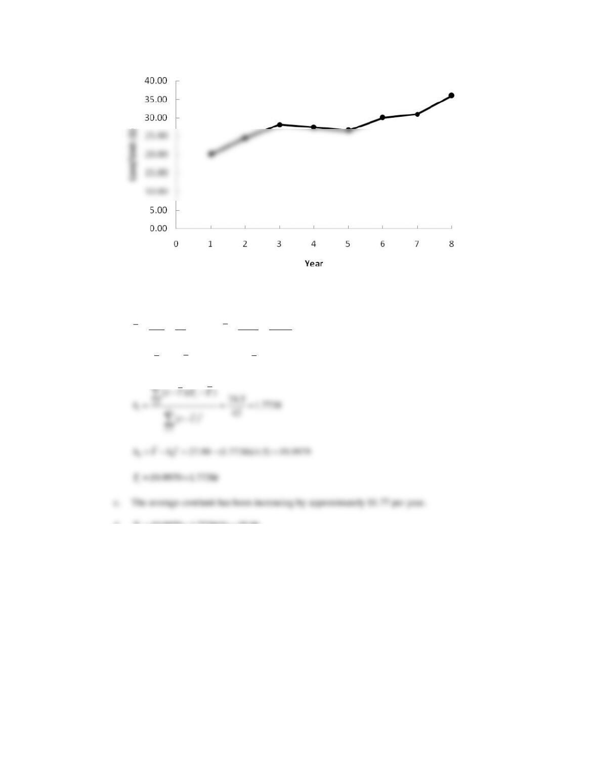
17. a.
The time series plot shows a linear trend.
b.
11
15 55
3 11
55
nn
t
tt
tY
tY
nn
==
= = = = = =
2
( )( ) 21 ( ) 10
t
t t Y Y t t − − = − =
1
( )( ) 21 2.1
n
t
tn
t t Y Y
=
−−
$0.0
$50.0
$100.0
$150.0
$200.0
$250.0
$300.0
2003 2005 2007 2009 2011 2013
Median Home Price ($000)
Year
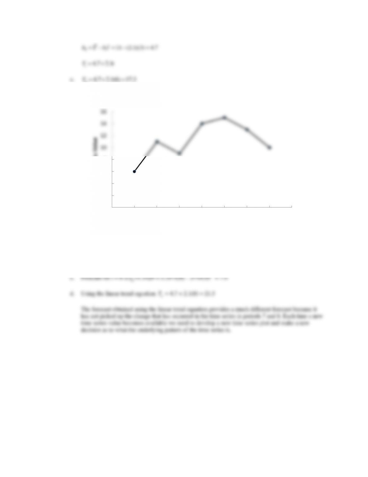
64.7 2.1(6) 17.3T= + =
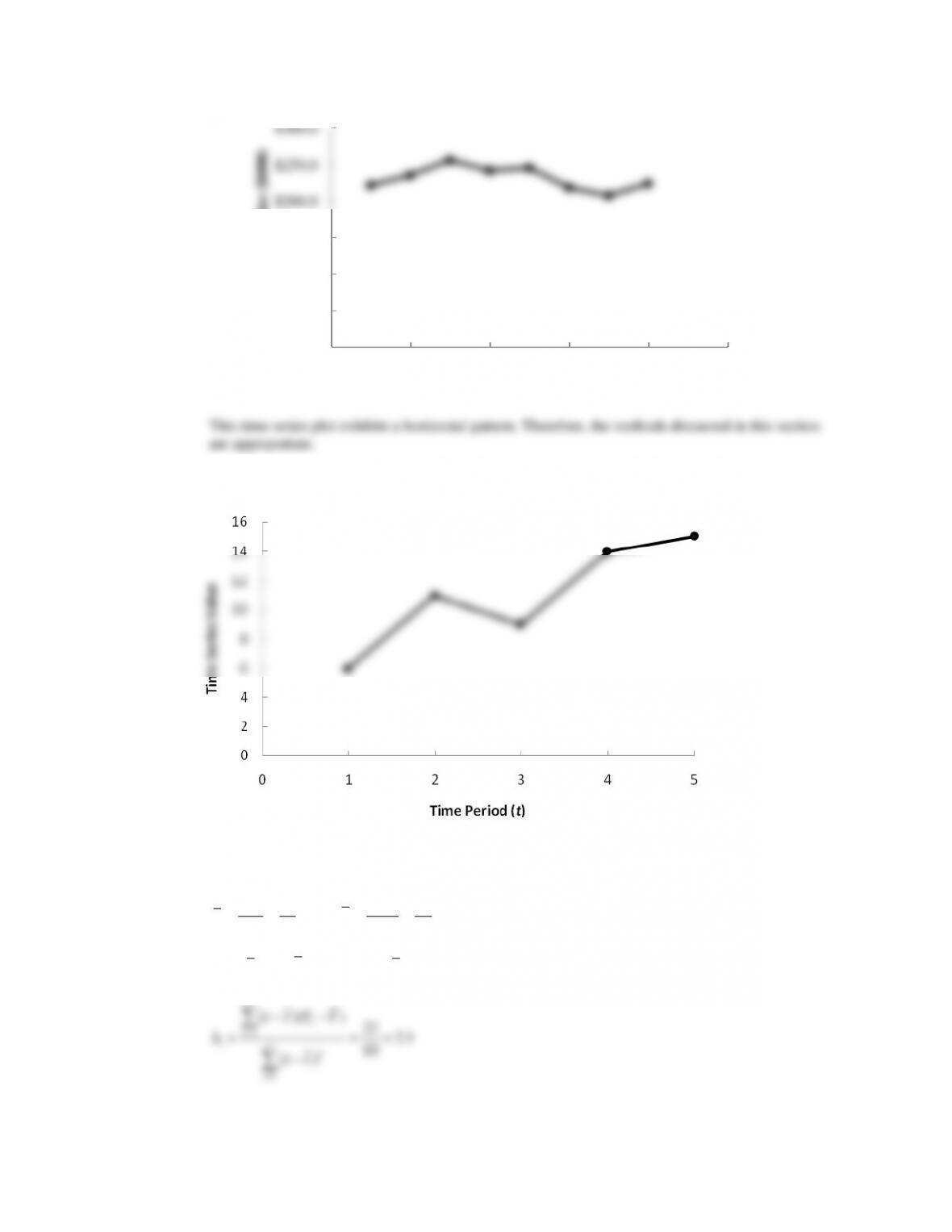
18. a.
The time series plot exhibits a curvilinear trend.
b. Using Excel’s chart tools the quadratic trend equation is
t
T
=1.1429 + 5.3571t – .5714
2
t
T
2
0
2
4
6
8
10
12
14
16
0 1 2 3 4 5 6 7 8
Time Series Value
Time Period (t)
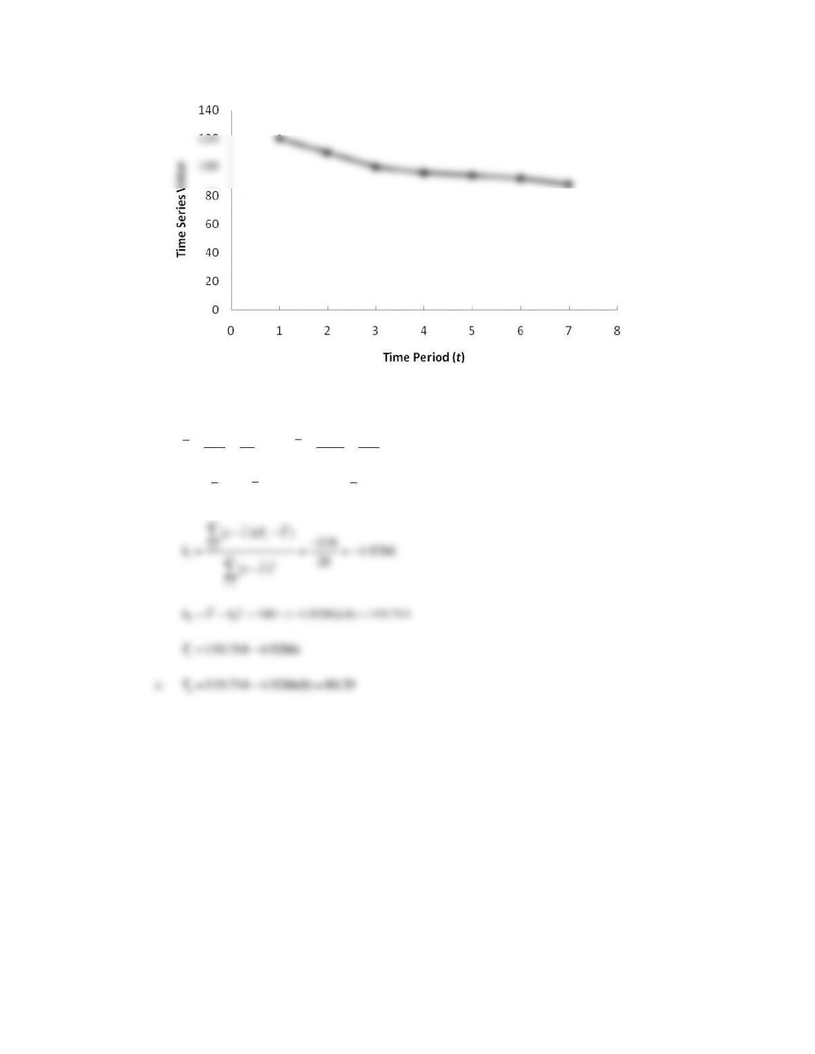
The time series plot shows a linear trend.
b.
11
28 700
4 100
77
nn
t
tt
tY
tY
nn
==
= = = = = =
2
( )( ) 138 ( ) 28
t
t t Y Y t t − − = − − =
1
( )( ) 138 4.9286
n
t
tn
t t Y Y
=
−−−
8119.714 4.9286(8) 80.29T= − =
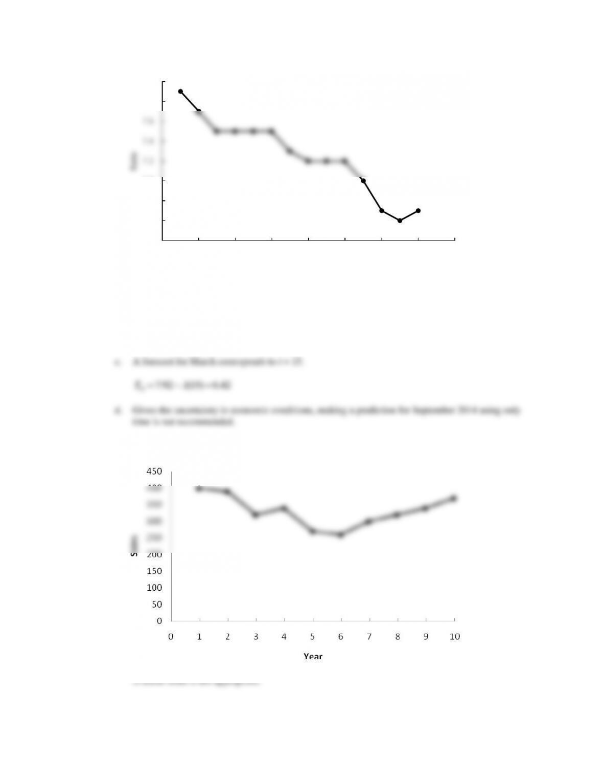
20. a.
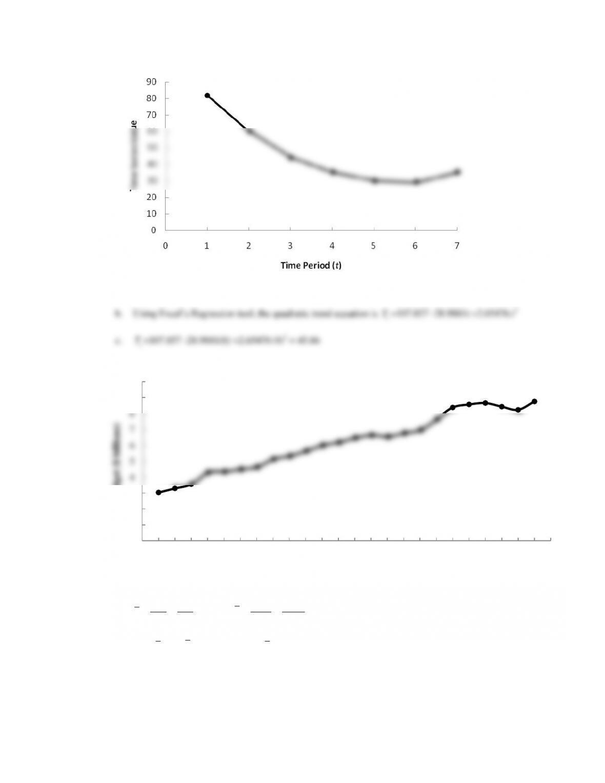
The time series plot exhibits a curvilinear trend.
t
2
t
21. a.
b.
11
300 148.2
12.5 6.175
24 24
nn
t
tt
tY
tY
nn
==
= = = = = =
2
( )( ) 290.86 ( ) 1150
t
t t Y Y t t − − = − =
0
1
2
3
4
5
6
7
8
9
10
0 1 2 3 4 5 6 7 8 9 10 11 12 13 14 15 16 17 18 19 20 21 22 23 24 25
Budget ($ billions)
Year
1
12
( )( ) 290.86 .25292
n
t
tn
t t Y Y
b
=
−−
= = =
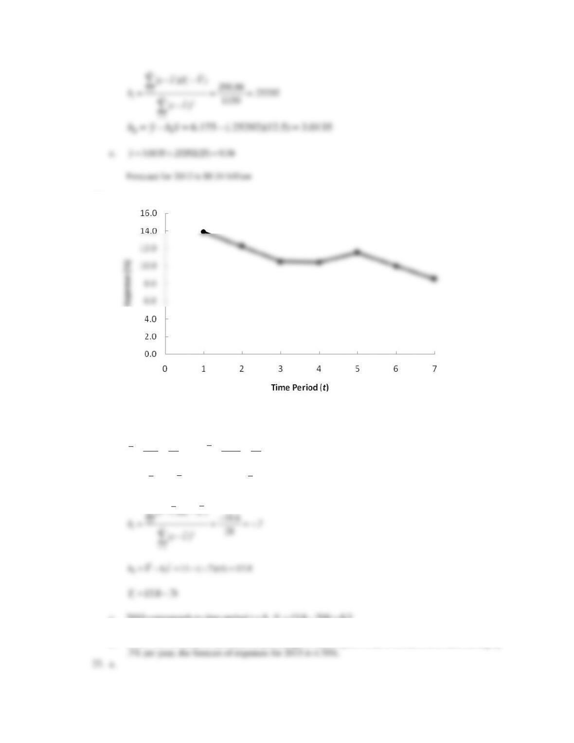
22. a.
The time series plot shows a downward linear trend
b.
11
28 77
4 11
77
nn
t
tt
tY
tY
nn
==
= = = = = =
2
( )( ) 19.6 ( ) 28
t
t t Y Y t t − − = − − =
1
( )( ) 19.6 .7
n
t
tn
t t Y Y
=
−−−
The time series plot shows an upward linear trend
b.
11
36 223.8
4.5 27.98
88
nn
t
tt
tY
tY
nn
==
= = = = = =
2
( )( ) 74.5 ( ) 42
t
t t Y Y t t − − = − =
1
( )( ) 74.5 1.7738
n
t
tn
t t Y Y
=
−−
The time series plot shows a linear trend.
b. Using Excel’s Regression tool, the linear trend equation is
7.92 .1
t
Tt=−
Note: t = 1 corresponds to January 2013, t = 2 corresponds to February 2013, and so on.
25. a.
A linear trend is not appropriate.
6.4
6.6
6.8
7.0
7.2
7.4
7.6
7.8
8.0
0246810 12 14 16
Rate
Period
b. Using Excel’s Regression tool, the quadratic trend equation is
2
472.7 62.9 5.303
t
T t t= − +
c.
2
11 472.7 62.9(11) 5.303(11) 422T= − + =
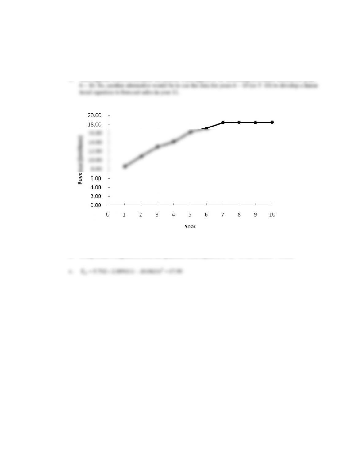
d. Sales appear to have bottomed-out in year 6 and appear to be increasing in a linear fashion for years
26. a.
A linear trend is not appropriate.
b. Using Excel’s Regression tool, the quadratic trend equation is
2
5.702 2.889 .1618
t
T t t= + −