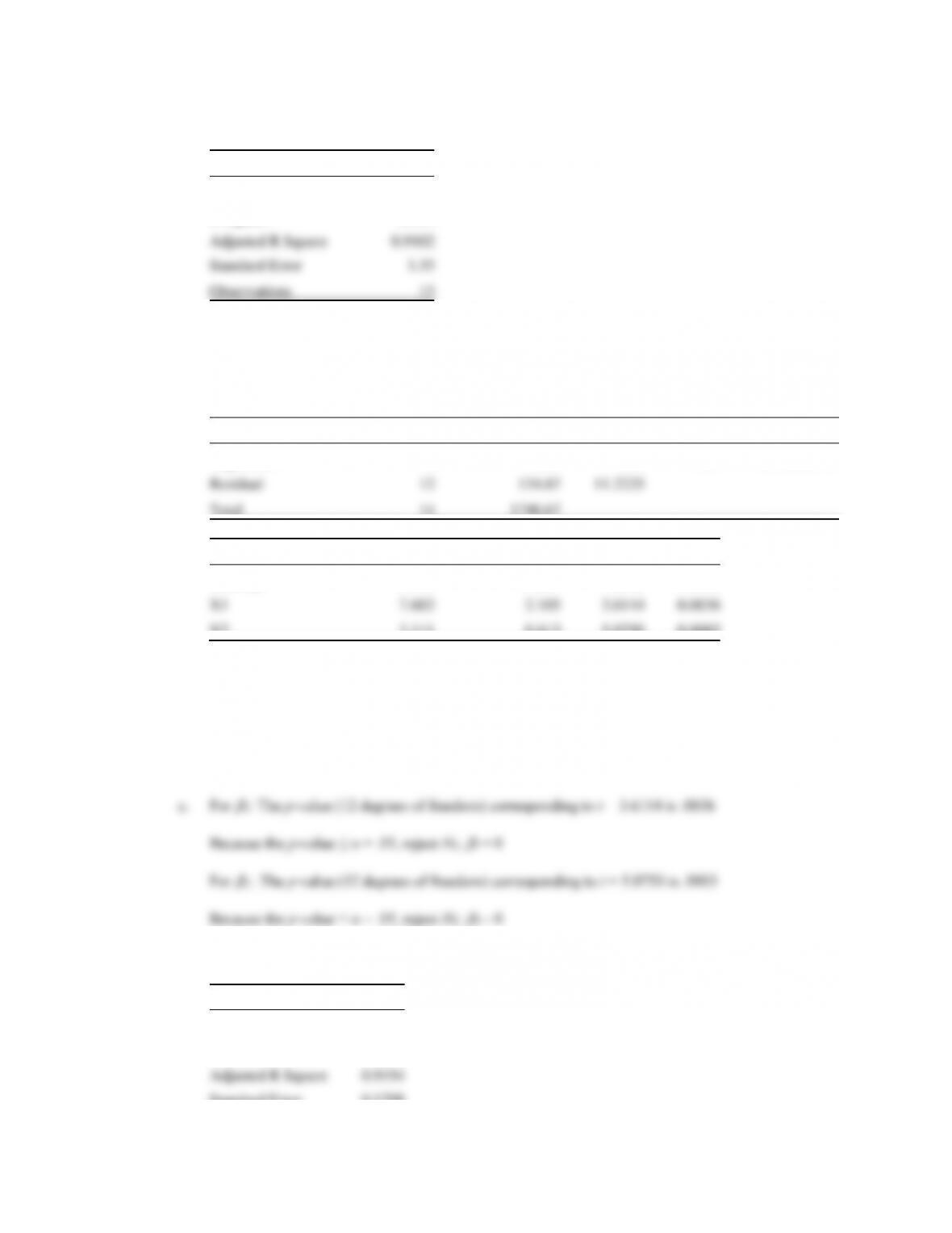
46. a. The computer output with the missing values filled in is as follows:
Regression Statistics
Multiple R
0.9607
R Square
0.923
Adjusted R Square
0.9102
Standard Error
3.35
Observations
15
ANOVA
df
SS
MS
F
Significance F
Regression
2
1612
806
71.82
2.10068E-07
Residual
12
134.67
11.2225
Total
14
1746.67
Coefficients
Standard Error
t Stat
P-value
Intercept
8.103
2.667
3.0382
0.0103
X1
7.602
2.105
3.6114
0.0036
X2
3.111
0.613
5.0750
0.0003
ˆ
y
= 8.103 + 7.602 X1 + 3.111 X2
b. The p-value (2 degrees of freedom numerator and 12 denominator) corresponding to F = 71.82 is
.0000
Because the p-value ≤ α = .05, there is a significant relationship.
47. a. The regression equation is
Regression Statistics
Multiple R
0.9681
R Square
0.9373
Adjusted R Square
0.9194
Standard Error
0.1298
Observations
10
ANOVA
df
SS
MS
F
Significance F
Regression
2
1.7621
0.8810
52.3053
6.17838E-05
Residual
7
0.1179
0.0168
Total
9
1.88
Coefficients
Standard Error
t Stat
P-value
Intercept
-1.4053
0.4848
-2.8987
0.0230
X1
0.0235
0.0087
2.7078
0.0303
X2
0.0049
0.0011
4.5125
0.0028
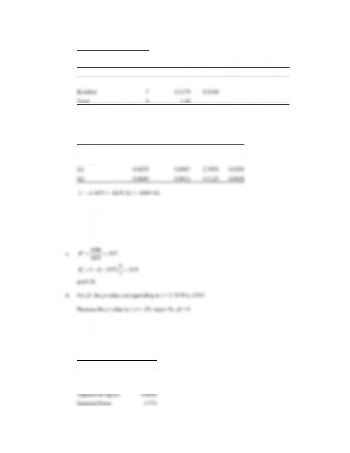
b. F = 52.3053
p-value (2 degrees of freedom numerator and 7 degrees of freedom denominator) = .0000
Because the p-value ≤ α = .05, there is a significant relationship.
2SSR .937
For
: the p-value corresponding to t = 4.5125 is .0028
Because the p-value is ≤ α = .05, reject H0:
= 0
48. a. The regression equation is
Regression Statistics
Multiple R
0.9493
R Square
0.9012
Adjusted R Square
0.8616
Standard Error
3.773
Observations
8
ANOVA
df
SS
MS
F
Significance F
Regression
2
648.83
324.415
22.7916
0.0031
Residual
5
71.17
14.234
Total
7
720
Coefficients
Standard Error
t Stat
P-value
Intercept
14.4
8.191
1.7580
0.1391
X1
-8.69
1.555
-5.5884
0.0025
X2
13.517
2.085
6.4830
0.0013
ˆ
y
= 14.4 – 8.69 X1 + 13.517 X2
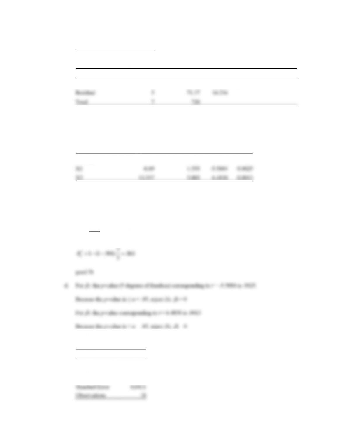
b. The p-value (5 degrees of freedom) corresponding to F = 22.7916 is .0031
Because the p-value is ≤ α = .05, there is a significant relationship.
c.
2SSR .901
SST
R==
27
49. a. A portion of the Excel output follows:
Regression Statistics
Multiple R
0.9182
R Square
0.8430
Adjusted R Square
0.8332
Standard Error
0.8411
Observations
18
ANOVA
df
SS
MS
F
Significance F
Regression
1
60.7866
60.7866
85.9295
7.80448E-08
Residual
16
11.3184
0.7074
Total
17
72.105
Coefficients
Standard Error
t Stat
P-value
Lower 95%
Upper 95%
Intercept
-7.5218
1.4668
-5.1282
0.0001
-10.6312
-4.4124
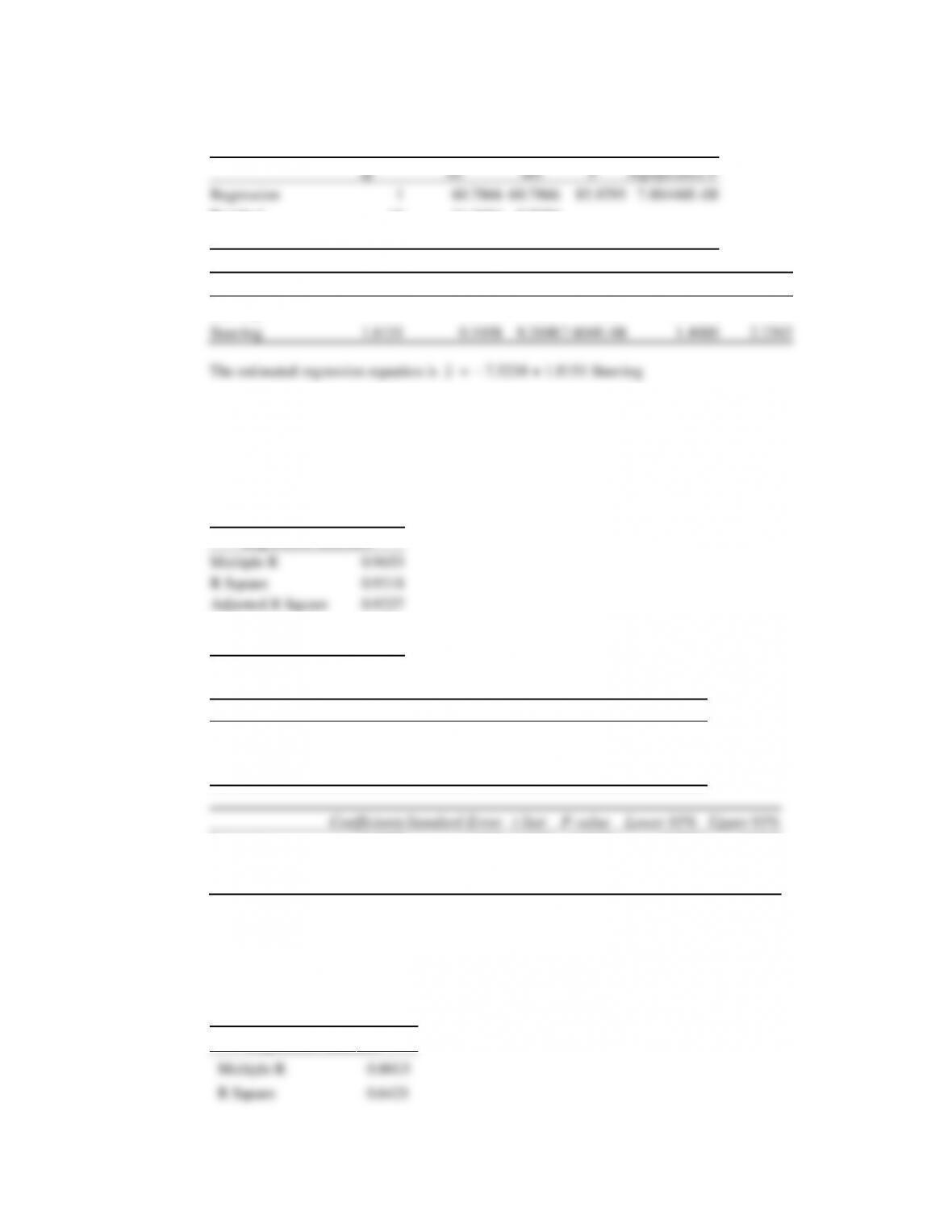
Steering
1.8151
0.1958
9.2698
7.804E-08
1.4000
2.2302
ˆ
y
Because the p-value = .000 < α = .05, there is a significant relationship.
b. The estimated regression equation provided a good fit; 84.3 % of the variability in the Buy Again
rating was explained by the linear effect of the Steering rating.
c. A portion of the Excel output follows:
Regression Statistics
Multiple R
0.9653
R Square
0.9318
Adjusted R Square
0.9227
Standard Error
0.5727
Observations
18
ANOVA
df
SS
MS
F
Significance F
Regression
2
67.1848
33.5924
102.4121
1.79936E-09
Residual
15
4.9202
0.3280
Total
17
72.105
Coefficients
Standard Error
t Stat
P-value
Lower 95%
Upper 95%
Intercept
-5.3877
1.1095
-4.8558
0.0002
-7.7526
-3.0228
Steering
0.6899
0.2875
2.3992
0.0299
0.0770
1.3028
Tread Wear
0.9113
0.2063
4.4166
0.0005
0.4715
1.3511
The estimated regression equation is
ˆ
y
= – 5.3877 + 0.6899 Steering + 0.9113 Treadwear
d. For the Treadwear independent variable, the p-value = .0005 < α = .05; thus, the addition of
Treadwear is significant.
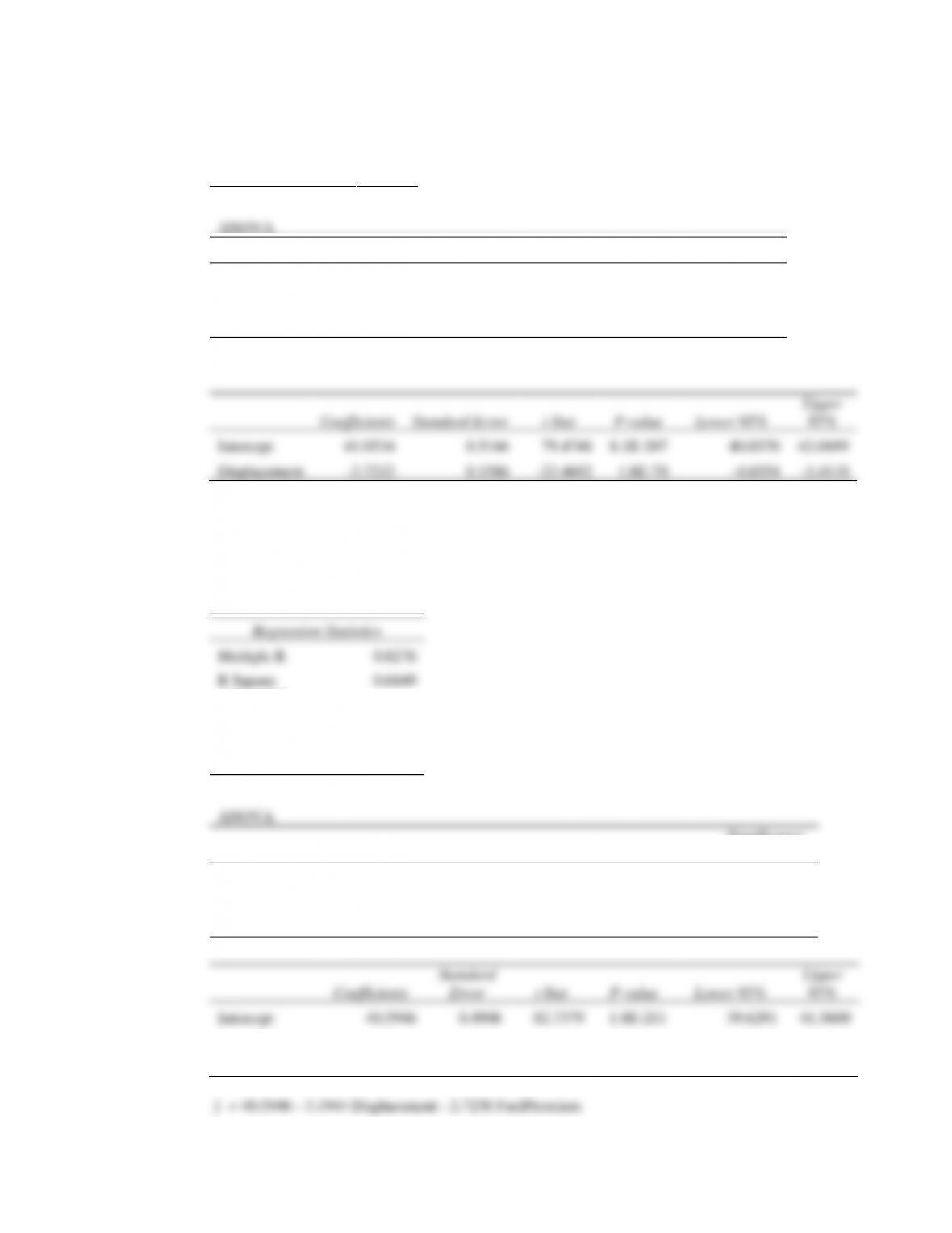
50. a. A portion of the Regression tool output follows.
Regression Statistics
Multiple R
0.8013
R Square
0.6421
Adjusted R Square
0.6409
Standard Error
3.4123
Observations
309
ANOVA
df
SS
MS
F
Significance F
Regression
1
6413.2883
6413.2883
550.8029
1.79552E-70
Residual
307
3574.5628
11.6435
Total
308
9987.8511
Coefficients
Standard Error
t Stat
P-value
Lower 95%
Upper
95%
Intercept
41.0534
0.5166
79.4748
8.1E-207
40.0370
42.0699
Displacement
-3.7232
0.1586
-23.4692
1.8E-70
-4.0354
-3.4110
ˆ
y
= 41.0534 ˗ 3.7232 Displacement
Because the p–value corresponding to F = 550.8029 is .0000 <
= .05, there is a significant
relationship.
b. A portion of the Excel Regression tool output follows.
Regression Statistics
Multiple R
0.8276
R Square
0.6849
Adjusted R
Square
0.6829
Standard Error
3.2068
Observations
309
ANOVA
df
SS
MS
F
Significance
F
Regression
2
6841.0876
3420.5438
332.6232
1.79466E-77
Residual
306
3146.7635
10.2835
Total
308
9987.8511
Coefficients
Standard
Error
t Stat
P-value
Lower 95%
Upper
95%
Intercept
40.5946
0.4906
82.7379
1.8E-211
39.6291
41.5600
Displacement
-3.1944
0.1701
-18.7745
7.43E-53
-3.5292
-2.8596
FuelPremium
-2.7230
0.4222
-6.4498
4.37E-10
-3.5537
-1.8922
ˆ
y

c. For FuelPremium, the p-value corresponding to t = -6.4498 is .000 < = .05; significant. The
addition of the dummy variables is significant.
d. A portion of the Excel Regression tool output follows.
ANOVA
df
SS
MS
F
Significance F
Regression
2
2096.8489
1048.4245
33.4584
2.03818E-09
Residual
42
1316.0771
31.3352
Total
44
3412.9260
Coefficients
Standard Error
t Stat
P-value
Lower 95%
Upper 95%
Intercept
4.9090
1.7702
2.7732
0.0082
1.3366
8.4814
FundDE
10.4658
2.0722
5.0505
9.033E-06
6.2839
14.6477
FundIE
21.6823
2.6553
8.1658
3.288E-10
16.3237
27.0408
The estimated regression equation is
ˆ
y
= 4.9090+ 10.4658 FundDE + 21.6823 FundIE
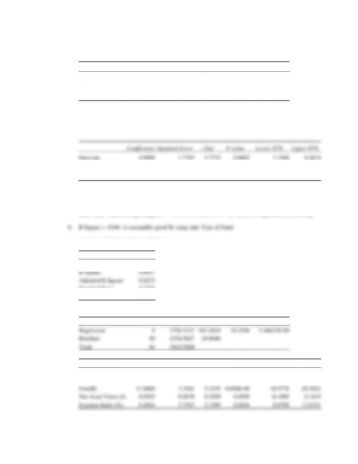
Since the p-value corresponding to F = 33.4584 is .0000 < α = .05, there is a significant relationship.
c. A portion of the Excel output follows:
Regression Statistics
Multiple R
0.8135
R Square
0.6617
Adjusted R Square
0.6279
Standard Error
5.3726
Observations
45
ANOVA
df
SS
MS
F
Significance F
Regression
4
2258.3432
564.5858
19.5598
5.48647E-09
Residual
40
1154.5827
28.8646
Total
44
3412.9260
Coefficients
Standard Error
t Stat
P-value
Lower 95%
Upper 95%
Intercept
1.1899
2.3781
0.5004
0.6196
-3.6164
5.9961
FundDE
6.8969
2.7651
2.4942
0.0169
1.3083
12.4854
FundIE
17.6800
3.3161
5.3315
4.096E-06
10.9778
24.3821
Net Asset Value ($)
0.0265
0.0670
0.3950
0.6950
-0.1089
0.1619
Expense Ratio (%)
6.4564
2.7593
2.3399
0.0244
0.8798
12.0331
ˆ
y
Since the p-value corresponding to F = 19.5558 is .0000 < α = .05, there is a significant relationship.
For Net Asset Value ($), the p-value corresponding to t = .3950 is .6950 > = .05, Net Asset Value
($) is not significant and can be deleted from the model.
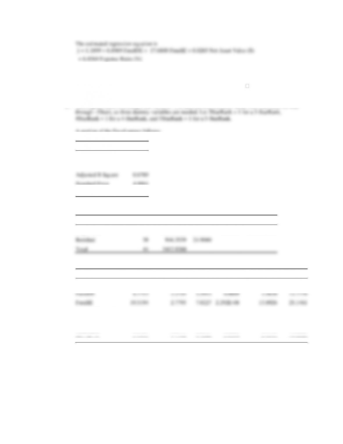
d. Morningstar Rank is a categorical variable. The data set only contains funds with four ranks (2-Star
Regression Statistics
Multiple R
0.8501
R Square
0.7227
Adjusted R Square
0.6789
Standard Error
4.9904
Observations
45
ANOVA
df
SS
MS
F
Significance F
Regression
6
2466.5721
411.0954
16.5072
2.96759E-09
Residual
38
946.3539
24.9040
Total
44
3412.9260
Coefficients
Standard Error
t Stat
P-value
Lower 95%
Upper 95%
Intercept
-4.6074
3.2909
-1.4000
0.1696
-11.2694
2.0547
FundDE
8.1713
2.2754
3.5912
0.0009
3.5650
12.7776
FundIE
19.5194
2.7795
7.0227
2.292E-08
13.8926
25.1461
Expense Ratio (%)
5.5197
2.5862
2.1343
0.0393
0.2843
10.7552
3StarRank
5.9237
2.8250
2.0969
0.0427
0.2048
11.6426
4StarRank
8.2367
2.8474
2.8927
0.0063
2.4725
14.0009
5StarRank
6.6241
3.1425
2.1079
0.0417
0.2624
12.9858
The estimated regression equation is
ˆ
y
= -4.6074 + 8.1713 FundDE + 19.5194 FundIE +5.5197 Expense Ratio (%) + 5.9237 3StarRank
+ 8.2367 4StarRank + 6.6241 5StarRank
At the .05 level of significance, all the independent variables are significant.

Total
29
7069.407
Coefficients
Standard Error
t Stat
P-value
Intercept
-407.9703
68.9533
-5.9166
4.18419E-06
FG%
4.9612
1.3676
3.6276
0.0013
3P%
2.3749
0.8074
2.9413
0.0071
FT%
0.0049
0.5182
0.0095
0.9925
RBOff
3.4612
1.3462
2.5711
0.0168
RBDef
3.6853
1.2965
2.8425
0.0090
ˆ
y
= ˗407.9703 + 4.9612 FG% + 2.3749 3P% + 0.0049 FT% + 3.4612 RBOff +
3.6853 RBDef
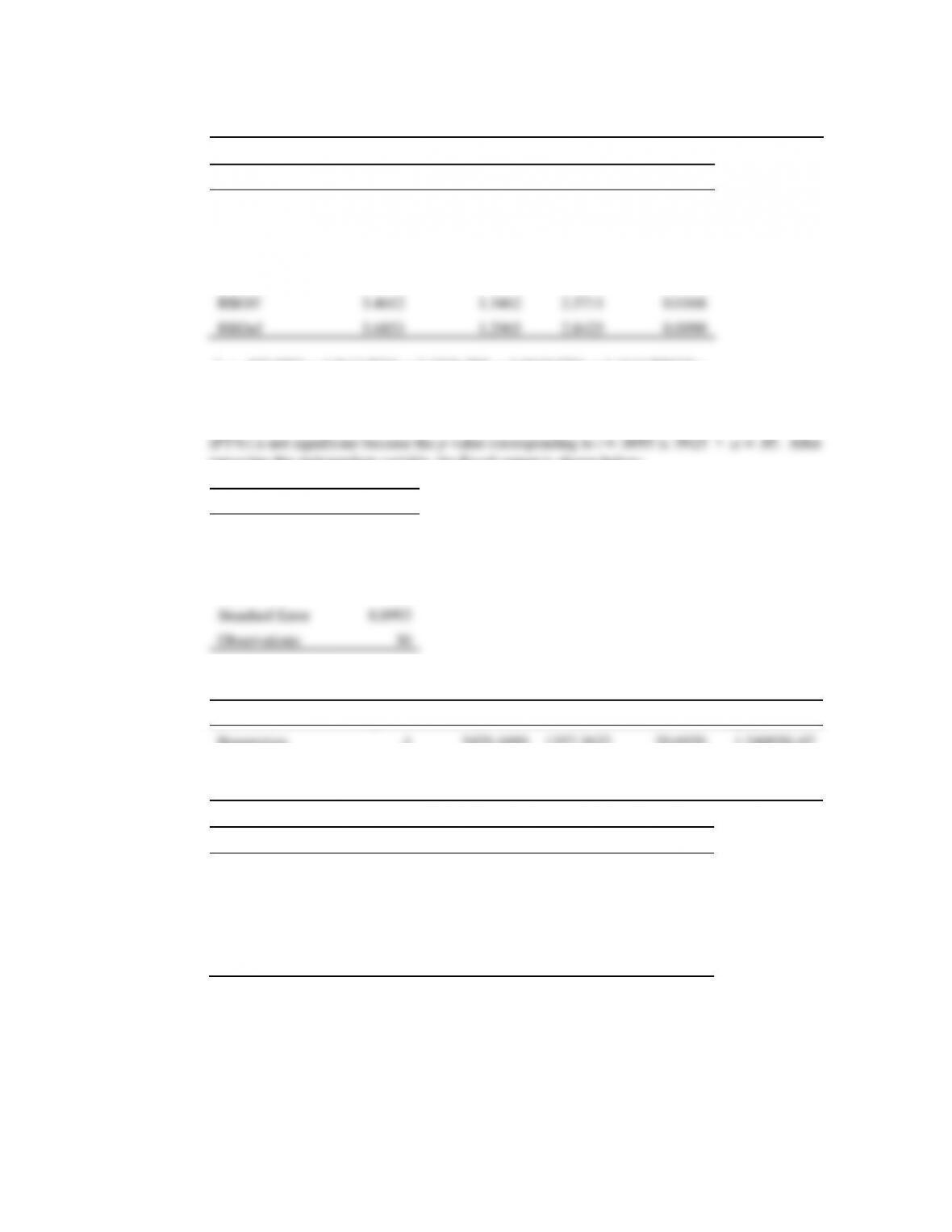
d. For the estimated regression equation developed in part (c), the percentage of free throws made
removing this independent variable, the Excel output is shown below:
Regression Statistics
Multiple R
0.8764
R Square
0.7680
Adjusted R
Square
0.7309
Standard Error
8.0993
Observations
30
ANOVA
df
SS
MS
F
Significance F
Regression
4
5429.4489
1357.3622
20.6920
1.24005E-07
Residual
25
1639.9581
65.5983
Total
29
7069.407
Coefficients
Standard Error
t Stat
P-value
Intercept
-407.5790
54.2152
-7.5178
7.1603E-08
FG%
4.9621
1.3366
3.7125
0.0010
3P%
2.3736
0.7808
3.0401
0.0055
RBOff
3.4579
1.2765
2.7089
0.0120
RBDef
3.6859
1.2689
2.9048
0.0076
ˆ
y
= –407.5790 + 4.9621 FG% + 2.3736 3P%+ 3.4579 RBOff + 3.6859 RBDef
e.
ˆ
y
= –407.5790 + 4.9621 FG% + 2.3736(35) + 3.4579(12) + 3.6859(30) = 50.86%