
10. a. A portion of the Excel output follows.
Regression Statistics
Multiple R
0.6477
R Square
0.4195
Adjusted R Square
0.3873
Standard Error
0.0603
Observations
20
ANOVA
df
SS
MS
F
Significance F
Regression
1
0.0473
0.0473
13.0099
0.0020
Residual
18
0.0654
0.0036
Total
19
0.1127
Coefficients
Standard Error
t Stat
P-value
Intercept
0.6758
0.0631
10.7135
3.06093E-09
SO/IP
-0.2838
0.0787
-3.6069
0.0020
ˆ
y
= 0.6758 ˗ 0.2838 SO/IP
b. A portion of the Excel output follows.
Regression Statistics
Multiple R
0.5063
R Square
0.2563
Adjusted R Square
0.2150
Standard Error
0.0682
Observations
20
ANOVA
df
SS
MS
F
Significance F
Regression
1
0.0289
0.0289
6.2035
0.0227
Residual
18
0.0838
0.0047
Total
19
0.1127
Coefficients
Standard Error
t Stat
P-value
Intercept
0.3081
0.0604
5.1039
7.41872E-05
HR/IP
1.3467
0.5407
2.4907
0.0227
ˆ
y
= 0.3081 + 1.3467 HR/IP
c. A portion of the Excel output follows.
Regression Statistics
Multiple R
0.7506
R Square
0.5635
Adjusted R Square
0.5121
Standard Error
0.0538
Observations
20
ANOVA
df
SS
MS
F
Significance F
Regression
2
0.0635
0.0317
10.9714
0.0009
Residual
17
0.0492
0.0029
Total
19
0.1127
Coefficients
Standard Error
t Stat
P-value
Intercept
0.5365
0.0814
6.5903
4.58698E-06
SO/IP
-0.2483
0.0718
–
3.4586
0.0030
HR/IP
1.0319
0.4359
2.3674
0.0300
ˆ
y
= 0.5365 ˗ 0.2483 SO/IP + 1.0319 HR/IP
The predicted value for R/IP was less than the actual value.
e. This suggestion does not make sense. If a pitcher gives up more runs per inning pitched this pitcher’s
earned run average also has to increase. For these data the sample correlation coefficient between
ERA and R/IP is .964.
SST 6,724.125
c.
22
1 10 1
1 (1 ) 1 (1 .924) .902
1 10 2 1
a
n
RR
np
−−
= − − = − − =
− − − −
d. The estimated regression equation provided an excellent fit.
2SSR 14,052.2 .926
Standard Error
2.8487
Observations
190
The value of R-Sq = 82.79% and the value of R-Sq (adj) = 82.60% indicate that the estimated
regression equation provided a very good fit.
b. A portion of the Excel output for part (b) of exercise 9 is shown below.
Regression Statistics
Multiple R
0.8647
R Square
0.7477
Adjusted R Square
0.7464
Standard Error
3.4394
Observations
190
variability in total distance. The addition of launch angle increases the percentage to almost 83%.
Therefore, the estimated regression equation using both ball speed and launch angle will provide
better predictions.
18. a. A portion of the Excel output for part (c) of exercise 10 is shown below.
Regression Statistics
Multiple R
0.7506
R Square
0.5635
Adjusted R Square
0.5121
Standard Error
0.0538
Observations
20
b. The fit is not great, but considering the nature of the data being able to explain slightly more than
50% of the variability in the number of runs given up per inning pitched using just two independent
variables is not too bad.
c. A portion of the Excel output for part using ERA as the dependent variable is shown below.
Regression Statistics
Multiple R
0.7907
R Square
0.6251
Adjusted R Square
0.5810
Standard Error
0.4272
Observations
20
ANOVA
df
SS
MS
F
Significance F
Regression
2
5.1739
2.5870
14.1750
0.0002
Residual
17
3.1025
0.1825
Total
19
8.2765
Coefficients
Standard Error
t Stat
P-value
Intercept
3.8781
0.6466
5.9976
1.44078E-05
SO/IP
-1.8428
0.5703
–
3.2310
0.0049
HR/IP
11.9933
3.4621
3.4641
0.0030
Approximately 60% of the variability in the ERA can be explained by the linear effect of HR/IP and
SO/IP. This is not too bad considering the complexity of predicting pitching performance.
19. a. MSR = SSR/p = 6,216.375/2 = 3,108.188
SSE 507.75
1 10 2 1np
− − − −
b. F = MSR/MSE = 3,108.188/72.536 = 42.85
p-value (2 degrees of freedom numerator and 7 denominator) = .0001
Because the p-value ≤ α = .05, the overall model is significant.
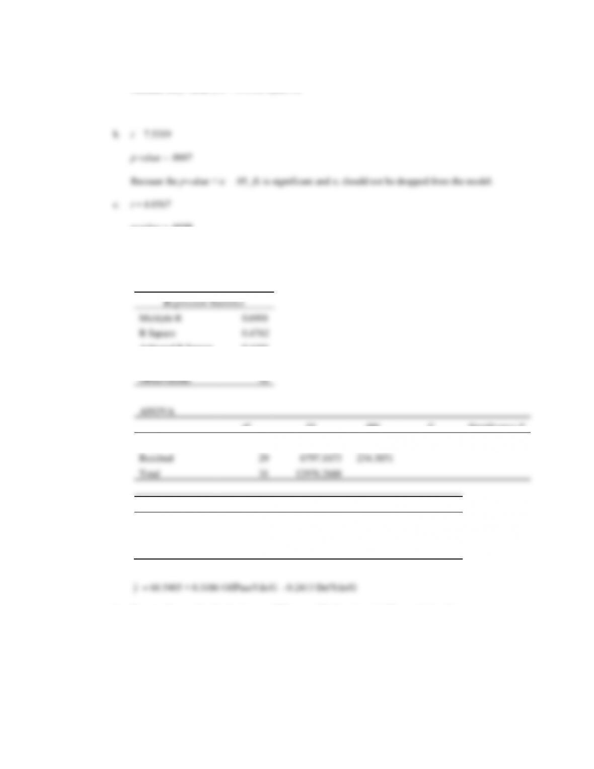
c. t = .5906/.0813 = 7.26
p-value (7 degrees of freedom) = .0002
Because the p-value ≤ α = .05,
is significant.
d. t = .4980/.0567 = 8.78
p-value (7 degrees of freedom) = .0001
Because the p-value ≤ α = .05,
is significant.
20. A portion of the Excel output is shown below.
Regression Statistics
Multiple R
0.9620
R Square
0.9255
Adjusted R Square
0.9042
Standard Error
12.7096
Observations
10
ANOVA
df
SS
MS
F
Significance F
Regression
2
14052.15497
7026.077
43.4957
0.0001
Residual
7
1130.745026
161.535
Total
9
15182.9
Coefficients
Standard Error
t Stat
P-value
Intercept
-18.36826758
17.97150328
-1.0221
0.3408
X1
2.0102
0.2471
8.1345
8.19E-05
X2
4.7378
0.9484
4.9954
0.0016
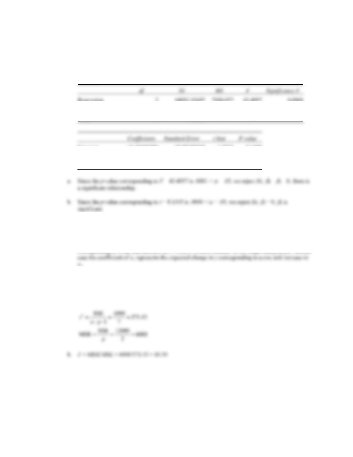
c. Since the p-value corresponding to t = 4.9954 is .0016 < = .05, we reject H0:
= 0;
is
significant.
21. a. In the two independent variable case the coefficient of x1 represents the expected change in y
corresponding to a one unit increase in x1 when x2 is held constant. In the single independent variable
b. Yes. If x1 and x2 are correlated, one would expect a change in the coefficient of x1 when x2 is
dropped from the model.
22. a. SSE = SST – SSR = 16000 – 12000 = 4000
p-value (2 degrees of freedom numerator and 7 denominator) = .0078
Because the p-value ≤ α = .05, we reject H0. There is a significant relationship among the variables.
23. a. F = 28.3778
p-value (2 degrees of freedom, numerator and 5 denominator) = .0019
Because the p-value ≤ α = .01, we reject H0.
p-value = .0098
Because the p-value ≤ α = .05,
is significant and x2 should not be dropped from the model.
24. a. A portion of the Excel output is shown below:
Regression Statistics
Multiple R
0.6901
R Square
0.4762
Adjusted R Square
0.4401
Standard Error
15.3096
Observations
32
ANOVA
df
SS
MS
F
Significance F
Regression
2
6179.1015
3089.5507
13.1815
8.47389E-05
Residual
29
6797.1673
234.3851
Total
31
12976.2688
Coefficients
Standard Error
t Stat
P-value
Intercept
60.5405
28.3562
2.1350
0.0413
OffPassYds/G
0.3186
0.0626
5.0929
1.95917E-05
DefYds/G
-0.2413
0.0893
-2.7031
0.0114
b. Because the p-value for the F test = .000 <
= .05, there is a significant relationship.
c. For OffPassYds/G: Because the p-value = .000 <
= .05, OffPassYds/G is significant.
For DefYds/G: Because the p-value = .0114 <
= .05, DefYds/G is significant.
25. a. A portion of the Excel output is shown below:

Regression Statistics
Multiple R
0.8659
R Square
0.7498
Adjusted R Square
0.7029
Standard Error
1.3877
Observations
20
ANOVA
df
SS
MS
F
Significance F
Regression
3
92.3520
30.7840
15.9847
4.51741E-05
Residual
16
30.8135
1.9258
Total
19
123.1655
Coefficients
Standard Error
t Stat
P-value
Intercept
35.6184
13.2308
2.6921
0.0160
Itineraries/Schedule
0.1105
0.1297
0.8519
0.4069
Shore Excursions
0.2445
0.0434
5.6400
3.68903E-05
Food/Dining
0.2474
0.0621
3.9821
0.0011
c. Itineraries/Schedule: Because the p-value = .4069 > α = .05, Itineraries/Schedule is significant.
For Shore Excursions: Because the p-value = .0000 <
= .05, Shore Excursions is significant.
For Food/Dining: Because the p-value = .0011 <
= .05, Food/Dining is significant.
Multiple R
0.8593
R Square
0.7385
Adjusted R Square
Standard Error
1.3765
ANOVA
df
SS
MS
Significance F
Regression
2
90.9545
45.4773
1.11912E-05
Residual
17
32.2110
1.8948
Total
19
123.1655
Coefficients
Standard Error
t Stat
Intercept
45.1780
6.9518
6.4987
5.458E-06
Shore Excursions
0.2529
0.0419
6.0369
1.334E-05
Food/Dining
0.2482
0.0616
4.0287
0.0009
The estimated regression equation is
ˆ
y
= 45.1780 ˗ 0.2529 Shore Excursions + 0.2482 Food/Dining
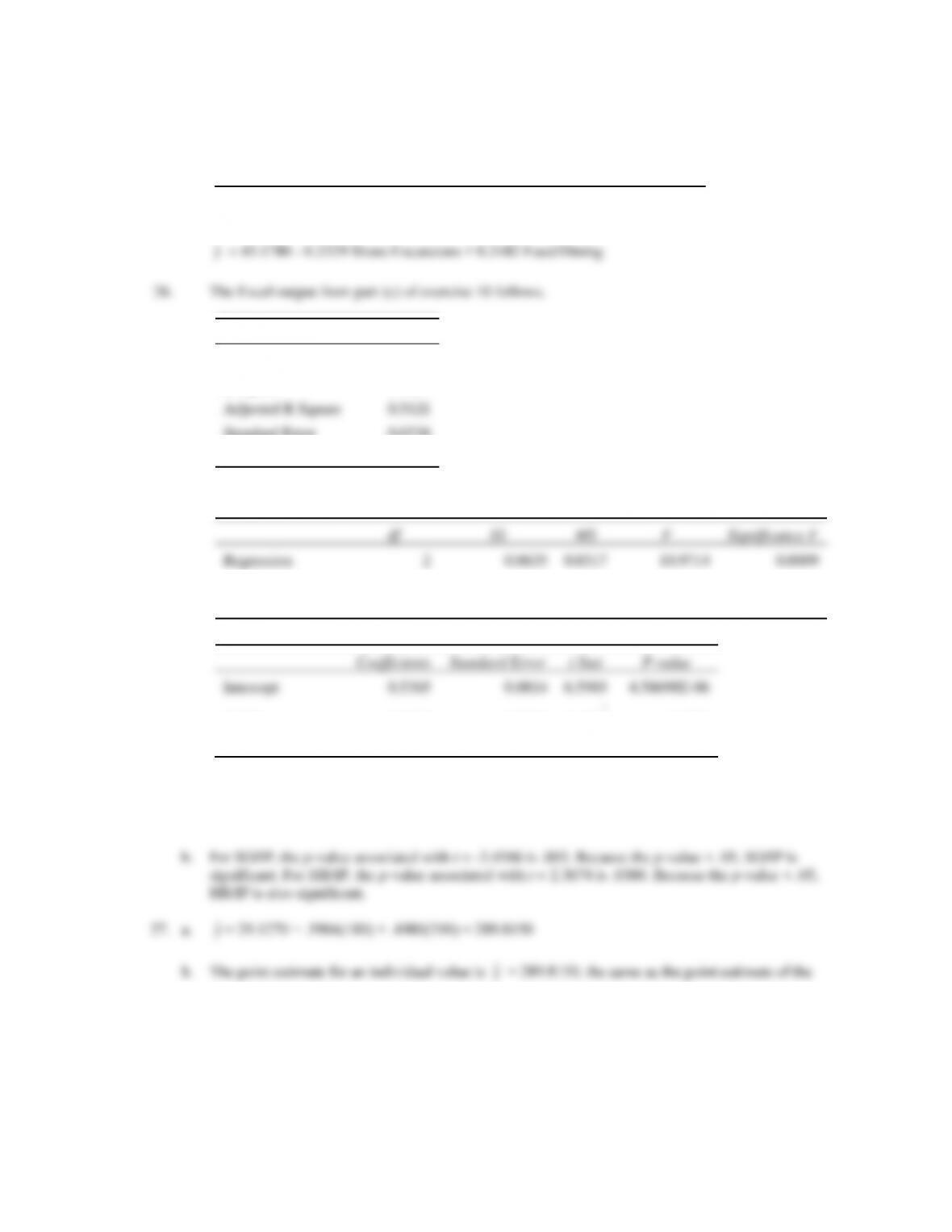
26. The Excel output from part (c) of exercise 10 follows.
Regression Statistics
Multiple R
0.7506
R Square
0.5635
Adjusted R Square
0.5121
Standard Error
0.0538
Observations
20
ANOVA
df
SS
MS
F
Significance F
Regression
2
0.0635
0.0317
10.9714
0.0009
Residual
17
0.0492
0.0029
Total
19
0.1127
Coefficients
Standard Error
t Stat
P-value
Intercept
0.5365
0.0814
6.5903
4.58698E-06
SO/IP
-0.2483
0.0718
–
3.4586
0.0030
HR/IP
1.0319
0.4359
2.3674
0.0300
a. The p-value associated with F = 10.9714 is .0009. Because the p-value < .05, there is a significant
overall relationship.
ˆ
y
ˆ
y
mean value.
28. a.
ˆ
y
= -18.4 + 2.01(45) + 4.74(15) = 143.15
b. Using StatTools, the 95% prediction interval is 111.16 to 175.16.
b. Using StatTools, the prediction interval estimate: 91.774 to 95.401 or $91,774 to $95,401
30. a. A portion of the Excel output form Exercise 24 is shown below:
Coefficients
Standard Error
t Stat
P-value
Intercept
60.5405
28.3562
2.1350
0.0413
OffPassYds/G
0.3186
0.0626
5.0929
1.95917E-05
DefYds/G
-0.2413
0.0893
-2.7031
0.0114
The estimated regression equation is
ˆ
y
= 60.5405 + 0.3186 OffPassYds/G ˗ 0.2413 DefYds/G
For OffPassYds/G = 225 and DefYds/G = 300, the predicted value of the percentage of games won
is
ˆ
y
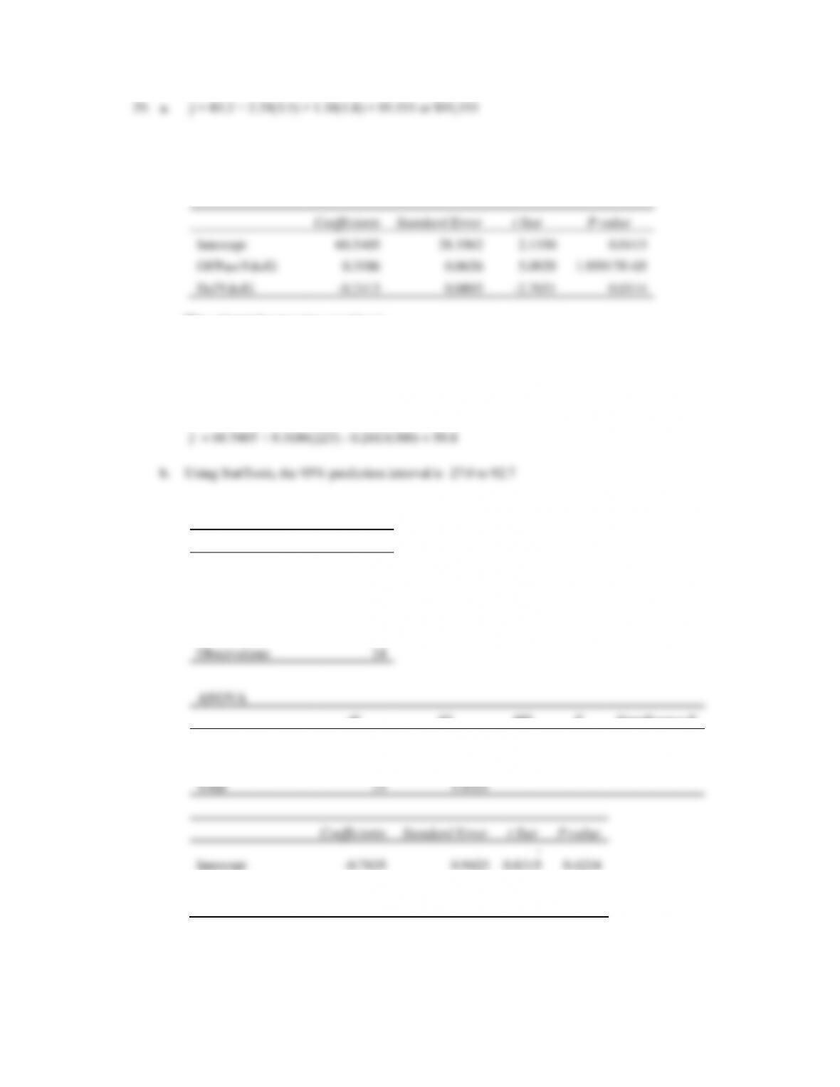
31. a. A portion of the Excel output is shown below:
Regression Statistics
Multiple R
0.8263
R Square
0.6827
Adjusted R Square
0.6250
Standard Error
0.4108
Observations
14
ANOVA
df
SS
MS
F
Significance F
Regression
2
3.9954
1.9977
11.8352
0.0018
Residual
11
1.8567
0.1688
Total
13
5.8521
Coefficients
Standard Error
t Stat
P-value
Intercept
-0.7835
0.9423
–
0.8315
0.4234
Trade Price
0.5580
0.2332
2.3929
0.0357
Speed of Execution
0.7342
0.1557
4.7142
0.0006
The estimated regression equation is
ˆ
y
= -0.7835 + 0.5580 Trade Price + 0.7342 Speed of Execution
b.
ˆ
y
= -0.7835 + 0.5580(3) + 0.7342(3) = 3.1
c. Using StatTools, the 95% prediction interval is 2.2 to 4.0