
Chapter 13
Multiple Regression
Learning Objectives
1. Understand how multiple regression analysis can be used to develop relationships involving one
dependent variable and several independent variables.
2. Be able to interpret the coefficients in a multiple regression analysis.
3. Know the assumptions necessary to conduct statistical tests involving the hypothesized regression
model.
4. Understand the role of Excel in performing multiple regression analysis.
5. Be able to interpret and use Excel’s Regression tool output to develop the estimated regression
equation.
6. Be able to determine how good a fit is provided by the estimated regression equation.
7. Be able to test for the significance of the regression equation.
8. Understand how multicollinearity affects multiple regression analysis.
Solutions:
1. a. b1 = .5906 is an estimate of the change in y corresponding to a 1 unit change in x1 when x2 is held
constant.
2. a. The Excel output is shown below:
Regression Statistics
Multiple R
0.8124
R Square
0.6600
Adjusted R Square
0.6175
Standard Error
25.4009
Observations
10
ANOVA
df
SS
MS
F
Significance F
Regression
1
10021.24739
10021.25
15.5318
0.0043
Residual
8
5161.652607
645.2066
Total
9
15182.9
Coefficients
Standard Error
t Stat
P-value
Intercept
45.0594
25.4181
1.7727
0.1142
X1
1.9436
0.4932
3.9410
0.0043
ˆ
y
b. The Excel output is shown below:
Regression Statistics
Multiple R
0.4707
R Square
0.2215
Adjusted R Square
0.1242
Standard Error
38.4374
Observations
10
ANOVA
df
SS
MS
F
Significance F
Regression
1
3363.4142
3363.414
2.2765
0.1698
Residual
8
11819.4858
1477.436
Total
9
15182.9
Coefficients
Standard Error
t Stat
P-value
Intercept
85.2171
38.3520
2.2220
0.0570
X2
4.3215
2.8642
1.5088
0.1698
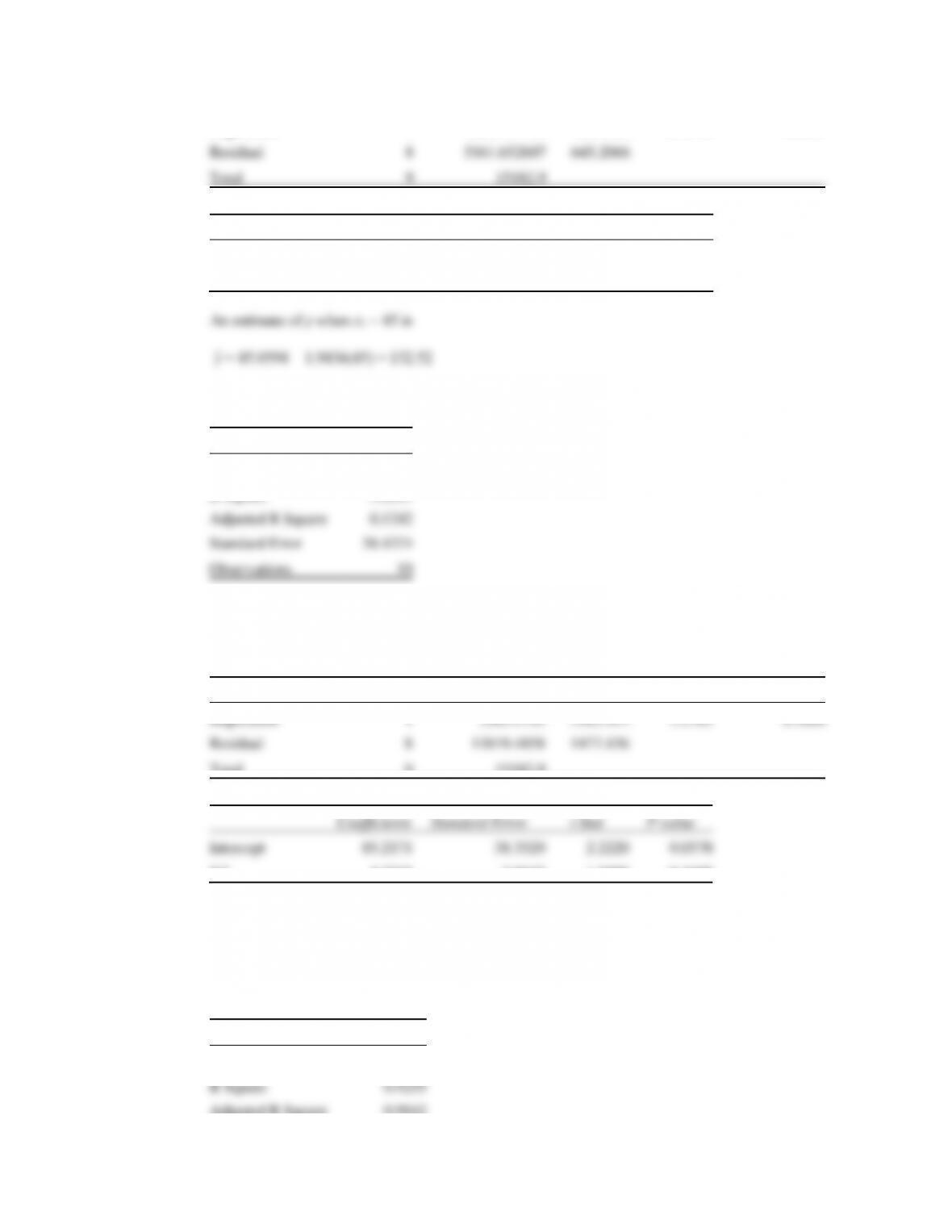
An estimate of y when x2 = 15 is
ˆ
y
= 85.2171 + 4.3215(15) = 150.04
c. The Excel output is shown below:
Regression Statistics
Multiple R
0.9620
R Square
0.9255
Adjusted R Square
0.9042
Standard Error
12.7096
Observations
10
ANOVA
df
SS
MS
F
Significance F
Regression
2
14052.15497
7026.077
43.4957
0.0001
Residual
7
1130.745026
161.535
Total
9
15182.9
Coefficients
Standard Error
t Stat
P-value
Intercept
-18.3683
17.97150328
-1.0221
0.3408
X1
2.0102
0.2471
8.1345
8.19E-05
X2
4.7378
0.9484
4.9954
0.0016
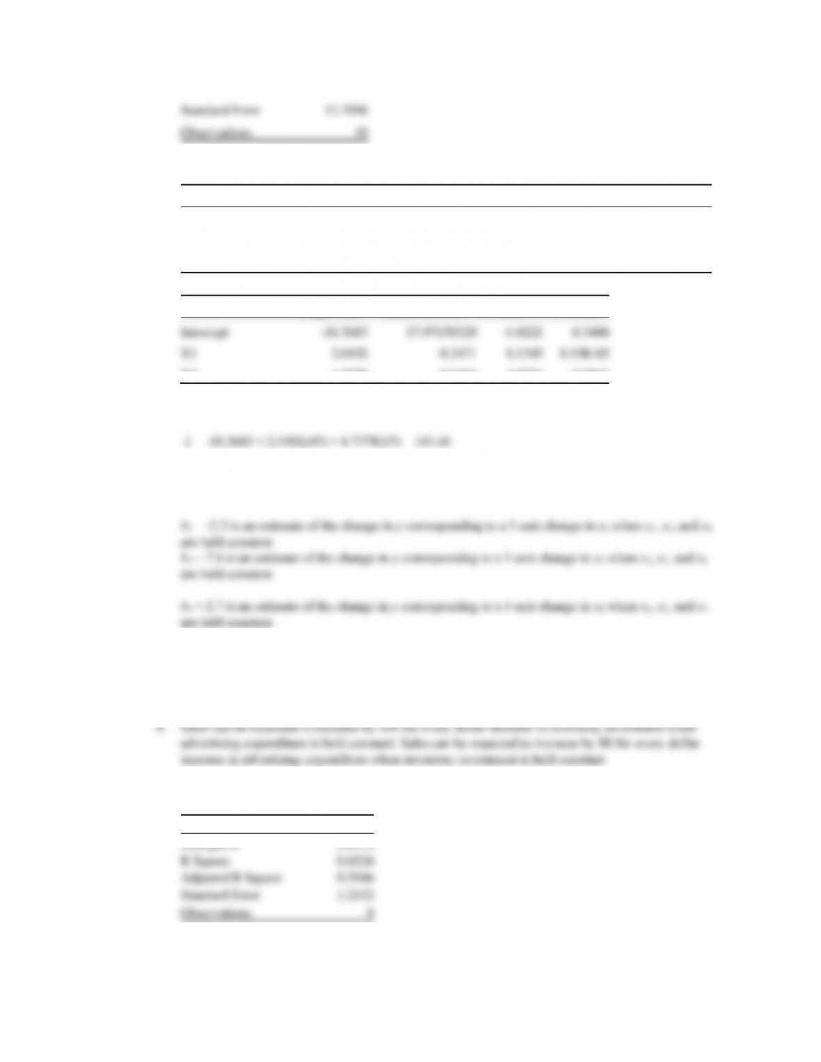
An estimate of y when x1 = 45 and x2 = 15 is
ˆ
y
3. a. b1 = 3.8 is an estimate of the change in y corresponding to a 1 unit change in x1 when x2, x3, and x4
are held constant.
b.
ˆ
y
= 17.6 + 3.8(10) – 2.3(5) + 7.6(1) + 2.7(2) = 57.1
4. a.
ˆ
y
= 25 + 10(15) + 8(10) = 255; sales estimate: $255,000
5. a. The Excel output is shown below:
Regression Statistics
Multiple R
0.8078
R Square
0.6526
Adjusted R Square
0.5946
Standard Error
1.2152
Observations
8
ANOVA
df
SS
MS
F
Significance F
Regression
1
16.6401
16.6401
11.2688
0.0153
Residual
6
8.8599
1.4767
Total
7
25.5
Coefficients
Standard Error
t Stat
P-value
Intercept
88.6377
1.5824
56.0159
2.174E-09
Television
Advertising ($1000s)
1.6039
0.4778
3.3569
0.0153
ˆ
y
= 88.6377 + 1.6039x1
where x1 = television advertising ($1000s)
b. The Excel output is shown below:
Regression Statistics
Multiple R
0.9587
R Square
0.9190
Adjusted R Square
0.8866
Standard Error
0.6426
Observations
8
ANOVA
df
SS
MS
F
Significance F
Regression
2
23.4354
11.7177
28.3778
0.0019
Residual
5
2.0646
0.4129
Total
7
25.5
Coefficients
Standard Error
t Stat
P-value
Intercept
83.2301
1.5739
52.8825
4.57E-08
Television
Advertising ($1000s)
2.2902
0.3041
7.5319
0.0007
Newspaper
Advertising ($1000s)
1.3010
0.3207
4.0567
0.0098
ˆ
y
= 83.2301 + 2.2902x1 + 1.3010x2
where
x1 = television advertising ($1000s)
x2 = newspaper advertising ($1000s)
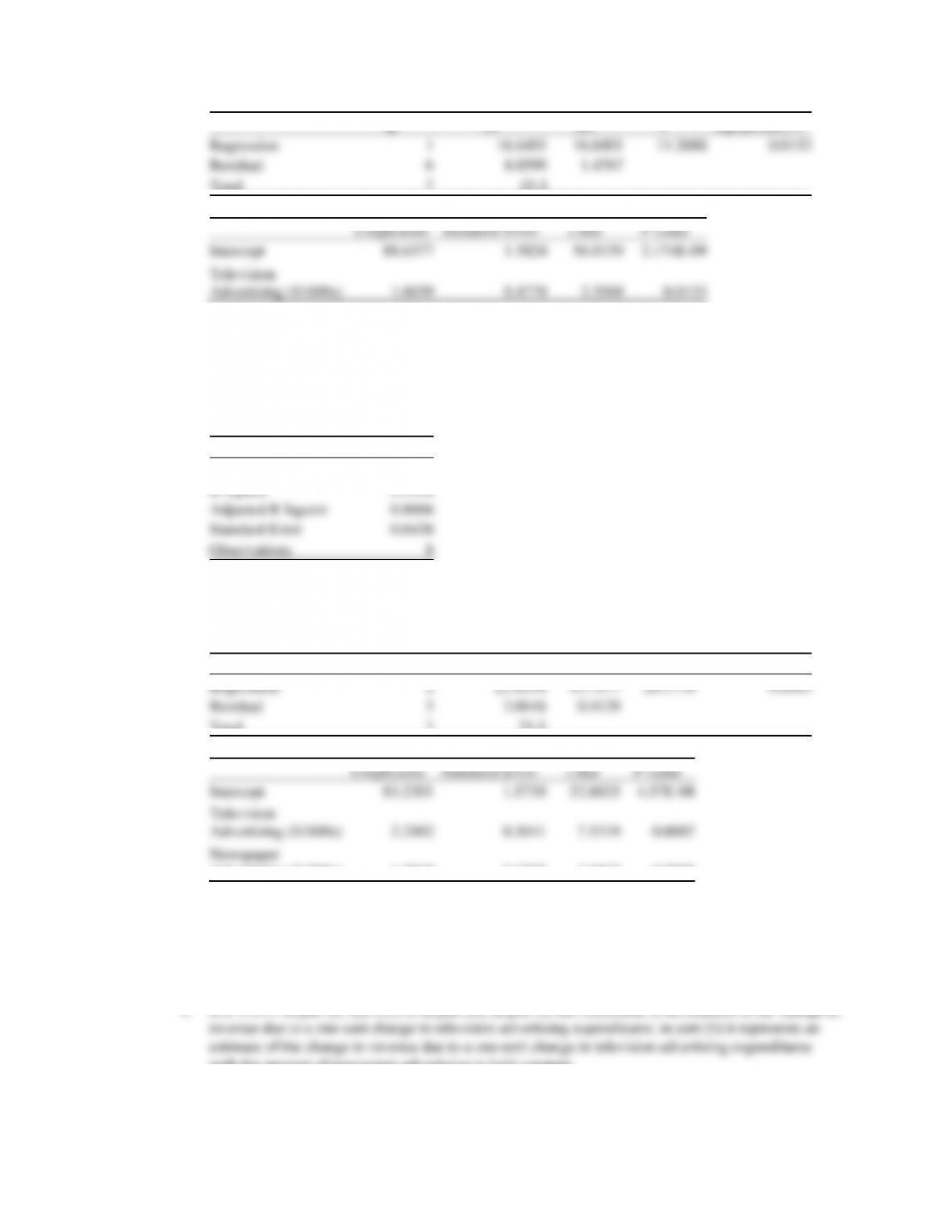
c. It is 1.6039 in part (a) and 2.2902 in part (b); in part (a) the coefficient is an estimate of the change in
with the amount of newspaper advertising is held constant
d. Revenue = 83.2301 + 2.2902(3.5) + 1.3010(1.8) = $93.59 or $93,590
6. a. A portion of the Excel output is shown below:
Regression Statistics
Multiple R
0.7597
R Square
0.5771
Adjusted R Square
0.5469
Standard Error
15.8732
Observations
16
ANOVA
df
SS
MS
F
Significance F
Regression
1
4814.2544
4814.2544
19.107
0.001
Residual
14
3527.4156
251.9583
Total
15
8341.67
Coefficients
Standard Error
t Stat
P-value
Intercept
-58.7703
26.1754
-2.2452
0.0414
Yds/Att
16.3906
3.7497
4.3712
0.0006
ˆ
y
= -58.7703 + 16.3906 Yds/Att
b. A portion of the Excel output is shown below:
Regression Statistics
Multiple R
0.6617
R Square
0.4379
Adjusted R Square
0.3977
Standard Error
18.3008
Observations
16
ANOVA
df
SS
MS
F
Significance F
Regression
1
3652.8003
3652.8003
10.9065
0.0052
Residual
14
4688.8697
334.9193
Total
15
8341.67
Coefficients
Standard Error
t Stat
P-value
Intercept
97.5383
13.8618
7.0365
5.898E-06
Int/Att
-1600.491
484.6300
-3.3025
0.0052
ˆ
y
= 97.5383 ˗ 1600.491 Int/Att
df
SS
MS
F
Significance F
Regression
1
66.3434
66.3434
9.8731
0.0138
Residual
8
53.7566
6.7196
Total
9
120.1
Coefficients
Standard Error
t Stat
P-value
Lower 95%
Upper 95%
Intercept
66.0623
3.7934
17.4153
1.2052E-07
57.3148
74.8098
Performance
0.1699
0.0541
3.1422
0.0138
0.0452
0.2946
The estimated regression equation is
ˆ
y
= 66.0623 + 0.1699 Performance
Multiple R
0.9148
R Square
0.8369
Adjusted R Square
0.7903
Standard Error
1.6729
Observations
df
SS
Significance F
Regression
2
17.9584
0.0018
Residual
7
19.5891
Total
9
120.1
Coefficients
Standard Error
P-value
Lower 95%
Upper 95%
Intercept
39.9820
7.8551
0.0014
21.4077
58.5562
Performance
0.1134
0.0385
0.0215
0.0224
0.2043
Features
0.3820
0.1093
0.0101
0.1235
0.6406
ˆ
y
Multiple R
0.6991
R Square
0.4888
Adjusted R Square
0.4604
Standard Error
1.8703
Observations
20
ANOVA
df
SS
MS
F
Significance F
Regression
1
60.2022
60.2022
17.2106
0.0006
Residual
18
62.9633
3.4980
Total
19
123.1655
Coefficients
Standard Error
t Stat
P-value
Intercept
69.2998
4.7995
14.4390
2.43489E-11
Shore Excursions
0.2348
0.0566
4.1486
0.0006
ˆ
y
= 69.2998 + 0.2348 Shore Excursions
Multiple R
R Square
Adjusted R Square
0.7077
Standard Error
Observations
20
ANOVA
df
SS
MS
F
Significance F
Regression
2
90.9545
45.4773
24.0015
0.0000
Residual
17
32.2110
1.8948
Total
19
123.1655
Coefficients
Standard Error
P-value
Intercept
45.1780
6.9518
6.4987
5.45765E-06
Shore Excursions
0.0419
6.0369
1.33357E-05
Food/Dining
0.0616
4.0287
ˆ
y
ˆ
y

Regression Statistics
Multiple R
0.8414
R Square
0.7080
Adjusted R Square
0.7064
Standard Error
3.7004
Observations
190
ANOVA
df
SS
MS
F
Significance F
Regression
1
6241.0689
6241.0689
455.7905
3.86529E-52
Residual
188
2574.2548
13.6928
Total
189
8815.3236
Coefficients
Standard Error
t Stat
P-value
Intercept
124.7160
7.4093
16.8325
2.24599E-39
Club Head Speed
1.3943
0.0653
21.3493
3.86529E-52
ˆ
y
= 124.7160 + 1.3943 Club Head Speed
b. A portion of the Excel output is shown below.
Regression Statistics
Multiple R
0.8647
R Square
0.7477
Adjusted R Square
0.7464
Standard Error
3.4394
Observations
190
ANOVA
df
SS
MS
F
Significance F
Regression
1
6591.4156
6591.4156
557.2110
4.0108E-58
Residual
188
2223.9081
11.8293
Total
189
8815.3236
Coefficients
Standard Error
t Stat
P-value
Intercept
117.1394
7.0221
16.6815
6.21713E-39
Ball Speed
0.9876
0.0418
23.6053
4.0108E–58
ˆ
y
= 117.1394 + 0.9876 Ball Speed
c. The following scatter diagram illustrates the relationship between the two variables.
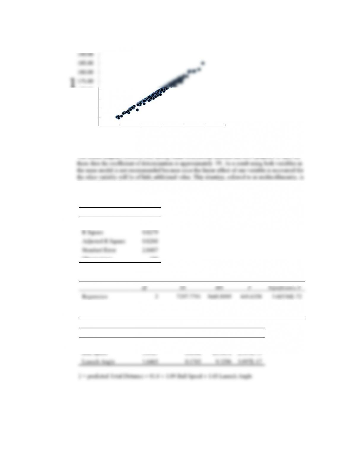
discussed later in the chapter in the section on testing for significance.
d. A portion of the Excel output is shown below.
Regression Statistics
Multiple R
0.9099
R Square
0.8279
Adjusted R Square
0.8260
Standard Error
2.8487
Observations
190
ANOVA
df
SS
MS
F
Significance F
Regression
2
7297.7791
3648.8895
449.6358
3.60536E-72
Residual
187
1517.5445
8.1152
Total
189
8815.3236
Coefficients
Standard Error
t Stat
P-value
Intercept
81.5964
6.9528
11.7357
3.458E-24
Ball Speed
1.0927
0.0364
29.9878
2.307E-73
Launch Angle
1.6465
0.1765
9.3296
3.097E-17
ˆ
y
e.
ˆ
y
= predicted Total Distance = 81.6 + 1.09 (170) + 1.65(11) = 285 yards
150.00
155.00
160.00
165.00
170.00
175.00
180.00
185.00
190.00
100.00 105.00 110.00 115.00 120.00 125.00 130.00
Ball Speed
Club Head Speed