Chapter 13
Multiple Regression
Case Problem 1: Consumer Research, Inc.
1. Descriptive statistics for these data are as follows:
Income
($1000s)
Household
Size
Amount
Charged ($)
Mean
43.48
Mean
3.42
Mean
3964.06
Standard Error
2.0578
Standard Error
0.2459
Standard Error
132.0160
Median
42
Median
3
Median
4090
Mode
54
Mode
2
Mode
3890
Standard Deviation
14.5507
Standard Deviation
1.7390
Standard Deviation
933.4941
Sample Variance
211.7241
Sample Variance
3.0241
Sample Variance
871411.2004
Kurtosis
-1.2477
Kurtosis
-0.7228
Kurtosis
-0.7418
Skewness
0.0959
Skewness
0.5279
Skewness
-0.1295
Range
46
Range
6
Range
3814
Minimum
21
Minimum
1
Minimum
1864
Maximum
67
Maximum
7
Maximum
5678
Sum
2174
Sum
171
Sum
198203
Count
50
Count
50
Count
50
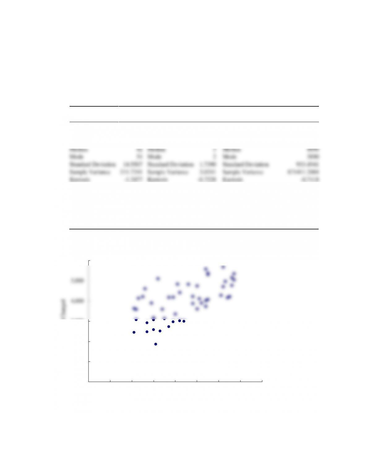
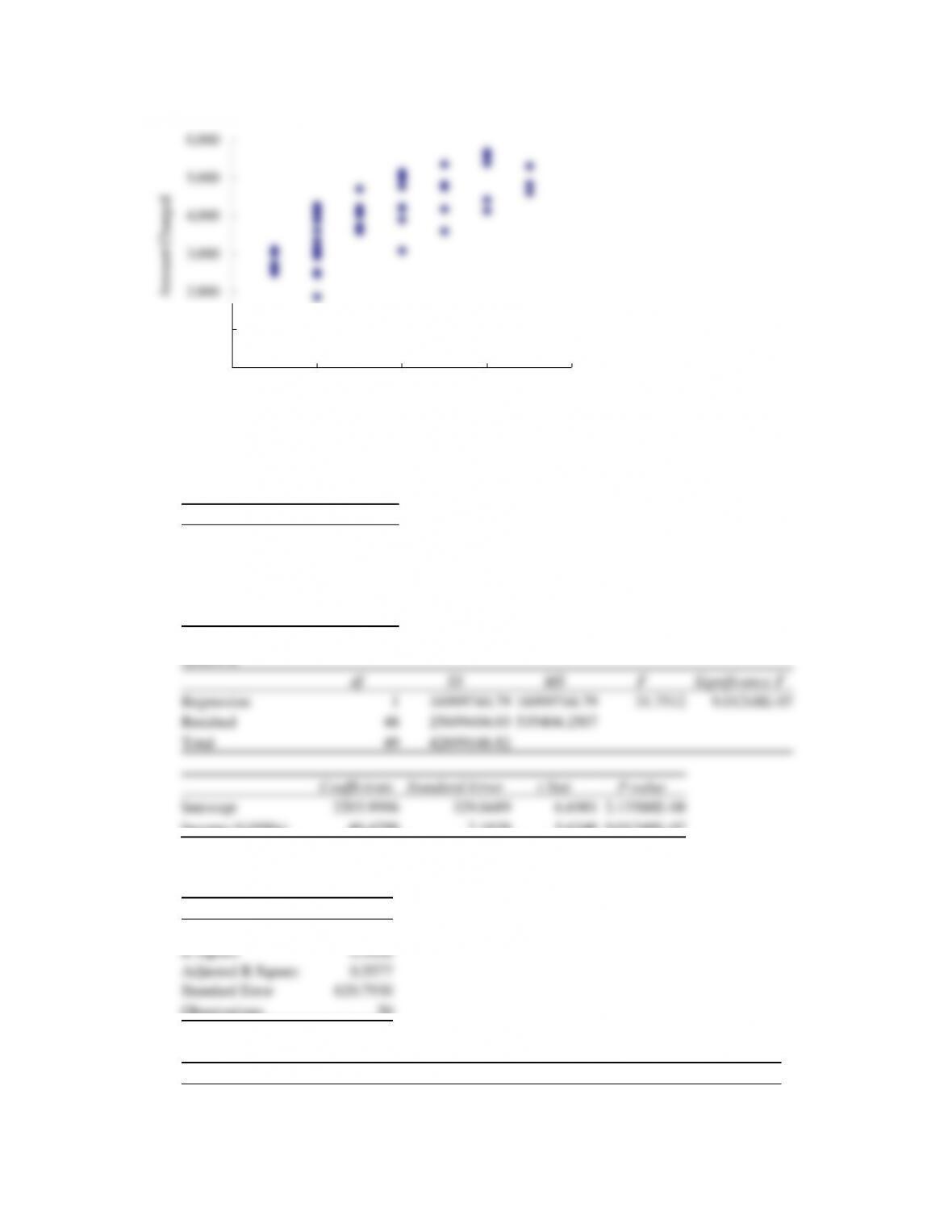
The following scatter diagrams suggest a linear relationship.
0
1,000
2,000
3,000
4,000
5,000
6,000
010 20 30 40 50 60 70 80
Amount Charged
Income
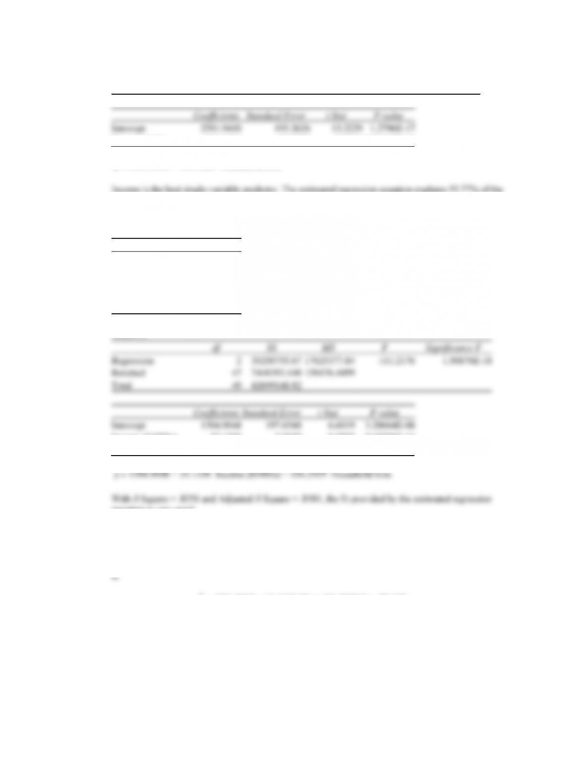
2. The estimated regression equations are shown below:
Regression Statistics
Multiple R
0.6310
R Square
0.3981
Adjusted R Square
0.3856
Standard Error
731.7132
Observations
50
ANOVA
df
SS
MS
F
Significance F
Regression
1
16999744.79
16999744.79
31.7512
9.01248E-07
Residual
48
25699404.03
535404.2507
Total
49
42699148.82
Coefficients
Standard Error
t Stat
P-value
Intercept
2203.9996
329.0489
6.6981
2.13588E-08
Income ($1000s)
40.4798
7.1839
5.6348
9.01248E-07
ˆ
y=
2203.9996 Income ($1000s)
Regression Statistics
Multiple R
0.7528
R Square
0.5668
Adjusted R Square
0.5577
Standard Error
620.7930
Observations
50
ANOVA
SS
MS
Significance F
Regression
1
24200717.48
24200717.48
62.7964
2.86495E-10
0
1,000
2,000
3,000
4,000
5,000
6,000
0 2 4 6 8
Amount Charged
Household Size
Residual
48
18498431.34
385383.9862
Total
49
42699148.82
Coefficients
Standard Error
t Stat
P-value
Intercept
2581.9410
195.2626
13.2229
1.2796E-17
Household Size
404.1284
50.9979
7.9244
2.86495E-10
ˆ
y=
2581.9410 + 404.1284 Household Size
Income is the best single-variable predictor. The estimated regression equation explains 55.77% of the
variability in the dependent variable.
3. The estimated regression equation using both independent variables is shown below:
Regression Statistics
Multiple R
0.9086
R Square
0.8256
Adjusted R Square
0.8181
Standard Error
398.0910
Observations
50
ANOVA
df
SS
MS
F
Significance F
Regression
2
35250755.67
17625377.84
111.2176
1.50876E-18
Residual
47
7448393.148
158476.4499
Total
49
42699148.82
Coefficients
Standard Error
t Stat
P-value
Intercept
1304.9048
197.6548
6.6019
3.28664E-08
Income ($1000s)
33.1330
3.9679
8.3503
7.68206E-11
Household Size
356.2959
33.2009
10.7315
3.12342E-14
ˆ
y=
equation is very good
4. The predicted annual credit card charge for a three-person household with an annual income of $40,000
ˆ
y
= 1304.9048 + 33.1330(40) + 356.2959(3) = $3,699
5. Other independent variables that could be added are age, gender, martial status, and whether the
consumer owns a home or rents.
Case Problem 2: Predicting Winnings for NASCAR Drivers
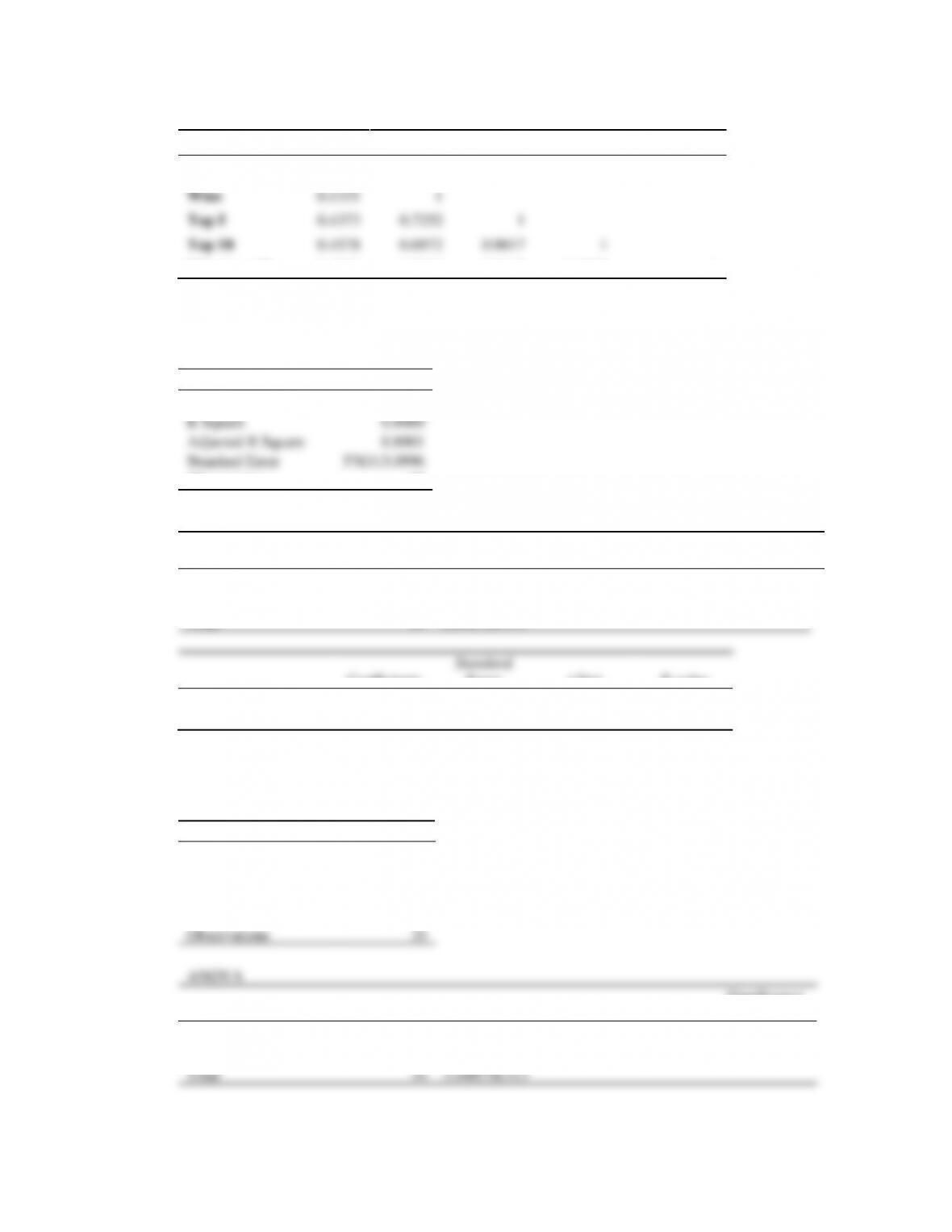
1. The Excel output showing the sample correlation coefficients follows.
Poles
Wins
Top 5
Top 10
Winnings ($)
Poles
1
Wins
0.1331
1
Top 5
0.4373
0.7252
1
Top 10
0.4578
0.6972
0.9017
1
Winnings ($)
0.4061
0.6616
0.8612
0.8978
1
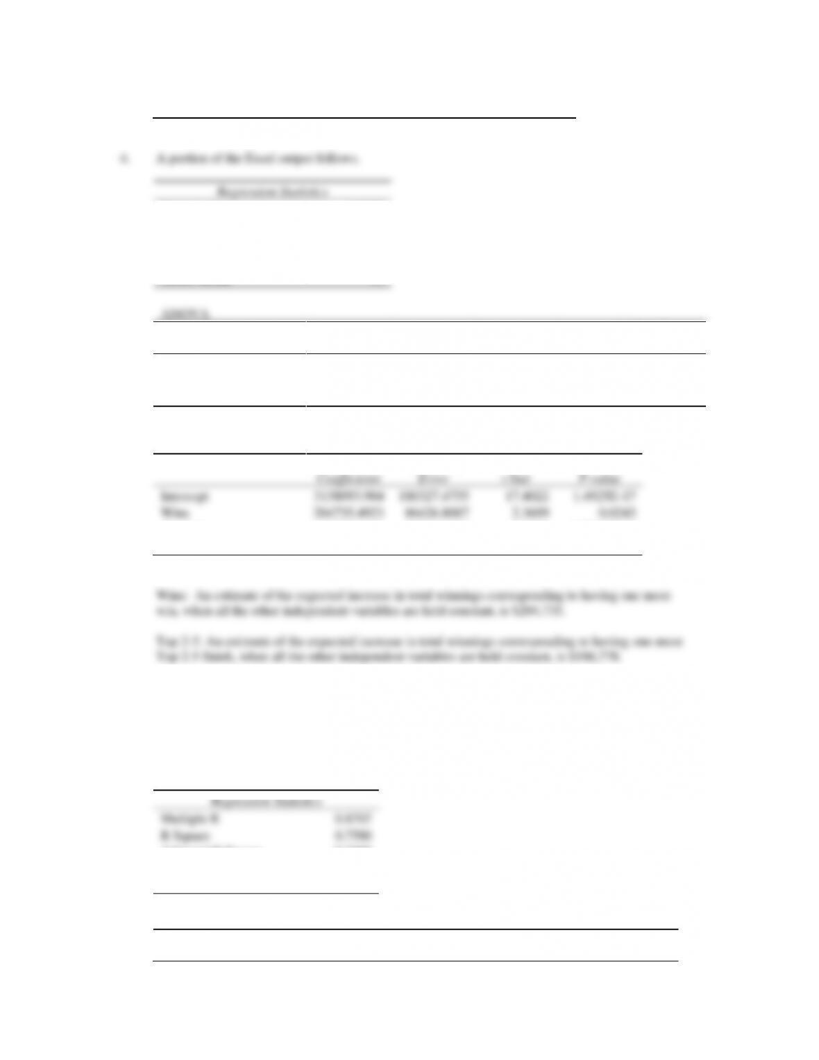
The variable most highly correlated with Winnings ($) is the number of top ten finishes. A portion
of the Excel output that uses the Top 10 independent variable to predict Winnings ($) follows.
Regression Statistics
Multiple R
0.8978
R Square
0.8060
Adjusted R Square
0.8001
Standard Error
576313.0996
Observations
35
ANOVA
df
SS
MS
F
Significance
F
Regression
1
4.5527E+13
4.5527E+13
137.0730
2.71202E-13
Residual
33
1.09605E+13
3.32137E+11
Total
34
5.64875E+13
Coefficients
Standard
Error
t Stat
P-value
Intercept
3049156.661
171768.9286
17.7515
1.89133E-18
Top 10
161934.0136
13831.2741
11.7078
2.71202E-13
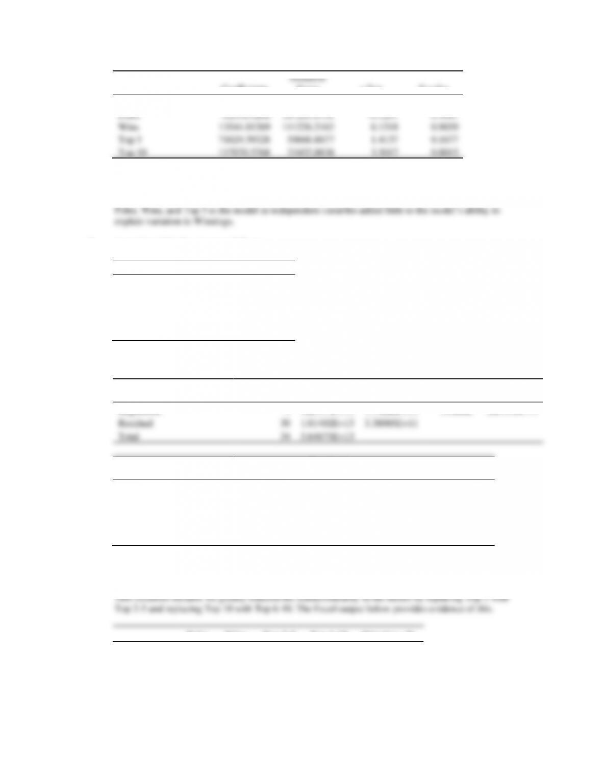
2. A portion of the Excel output follows.
Regression Statistics
Multiple R
0.9058
R Square
0.8205
Adjusted R Square
0.7966
Standard Error
581382.1968
Observations
35
ANOVA
df
SS
MS
F
Significance
F
Regression
4
4.63473E+13
1.15868E+13
34.2800
8.61942E-11
Residual
30
1.01402E+13
3.38005E+11
Total
34
5.64875E+13
Coefficients
Standard
Error
t Stat
P-value
Intercept
3140367.087
184229.0243
17.0460
5.5945E-17
Poles
-12938.9208
107205.0751
-0.1207
0.9047
Wins
13544.81269
111226.2163
0.1218
0.9039
Top 5
71629.39328
50666.8677
1.4137
0.1677
Top 10
117070.5768
33432.8838
3.5017
0.0015
Looking at the p-values corresponding to the t values for each of the independent variables, the only
significant variable is Top 10, with a p-value of .0015. Also note that this model has an R2 of 0.8205,
while the model that included only Top 10 as an independent variable had an R2 of .8060. Adding
3. A portion of the Excel output follows.
Regression Statistics
Multiple R
0.9058
R Square
0.8205
Adjusted R Square
0.7966
Standard Error
581382.1968
Observations
35
ANOVA
df
SS
MS
F
Significance
F
Regression
4
4.63473E+13
1.15868E+13
34.2800
8.61942E-11
Residual
30
1.01402E+13
3.38005E+11
Total
34
5.64875E+13
Coefficients
Standard
Error
t Stat
P-value
Intercept
3140367.087
184229.0243
17.0460
5.59454E-17
Poles
-12938.9208
107205.0751
-0.1207
0.9047
Wins
202244.7828
90225.8683
2.2415
0.0325
Top 2-5
188699.9701
34586.3223
5.4559
6.43028E-06
Top 6-10
117070.5768
33432.8838
3.5017
0.0015
Looking at the p-values corresponding to the t values for each of the independent variables, the only
independent variable that is not significant is Poles, with a p-value of .9047.
Poles
Wins
Top 2-5
Top 6-10
Winnings ($)
Poles
1
Wins
0.1331
1
Top 2-5
0.4889
0.5372
1
Top 6-10
0.3301
0.4197
0.4111
1
Multiple R
R Square
Adjusted R Square
Standard Error
Observations
Regression
1.5447E+13
Residual
3.2726E+11
Total
Intercept
Wins
Top 2-5
Top 6-10
Multiple R
R Square
Adjusted R Square
Standard Error
Observations
Winnings ($)
0.4061
0.6616
0.8226
0.6422
1
Multiple R
0.9671
R Square
0.9353
Adjusted R Square
0.9286
Standard Error
0.0720
Observations
54
Regression
0.7193
Residual
48
0.0052
Total
53
Coefficients
Intercept
1.3710
Cost/Mile
Road-Test Score
0.0111
Predicted Reliability
0.1662
Family-Sedan
0.0228
0.5516
Upscale-Sedan
0.0681
0.2108
Multiple R
0.9656
R Square
0.9324
Adjusted R Square
0.9283
Regression
2
0.4325
0.2163
79.8884
1.93001E-16
Residual
51
0.1381
0.0027
Total
53
0.5706
Coefficients
Standard
Error
t Stat
P-value
Intercept
0.5231
0.0144
36.2479
4.48609E-38
Family-Sedan
0.1189
0.0185
6.4157
4.55557E-08
Upscale-Sedan
0.2303
0.0184
12.5400
3.33718E-17
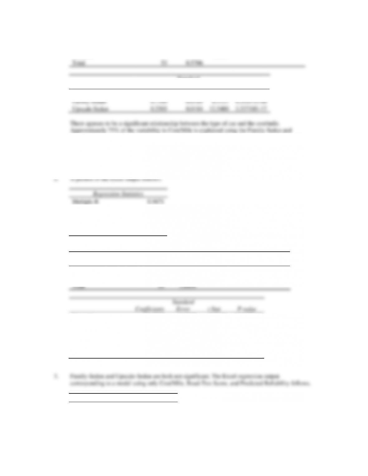
Upscale-Sedan variables. Note that for a small sedan, Family-Sedan = 0 and Upscale-Sedan = 1.
Thus the estimate of the Cost/Mile for a small sedan is .5231. Note that the Cost/Mile increases by
.1189 for a family sedan and .2303 for an upscale sedan. Conclusion: smaller cars have lower five–
year owner costs.
Standard Error
0.0721
Observations
54
ANOVA
df
SS
MS
F
Significance F
Regression
3
3.5853
1.1951
229.7327
3.15121E-29
Residual
50
0.2601
0.0052
Total
53
3.8454
Coefficients
Standard
Error
t Stat
P-value
Intercept
1.2444
0.0927
13.4202
3.36819E-18
Cost/Mile
-2.0433
0.1047
-19.5138
4.93912E-25
Road-Test Score
0.0114
0.0012
9.2522
2.05531E-12
Predicted Reliability
0.1651
0.0102
16.2574
1.33922E-21
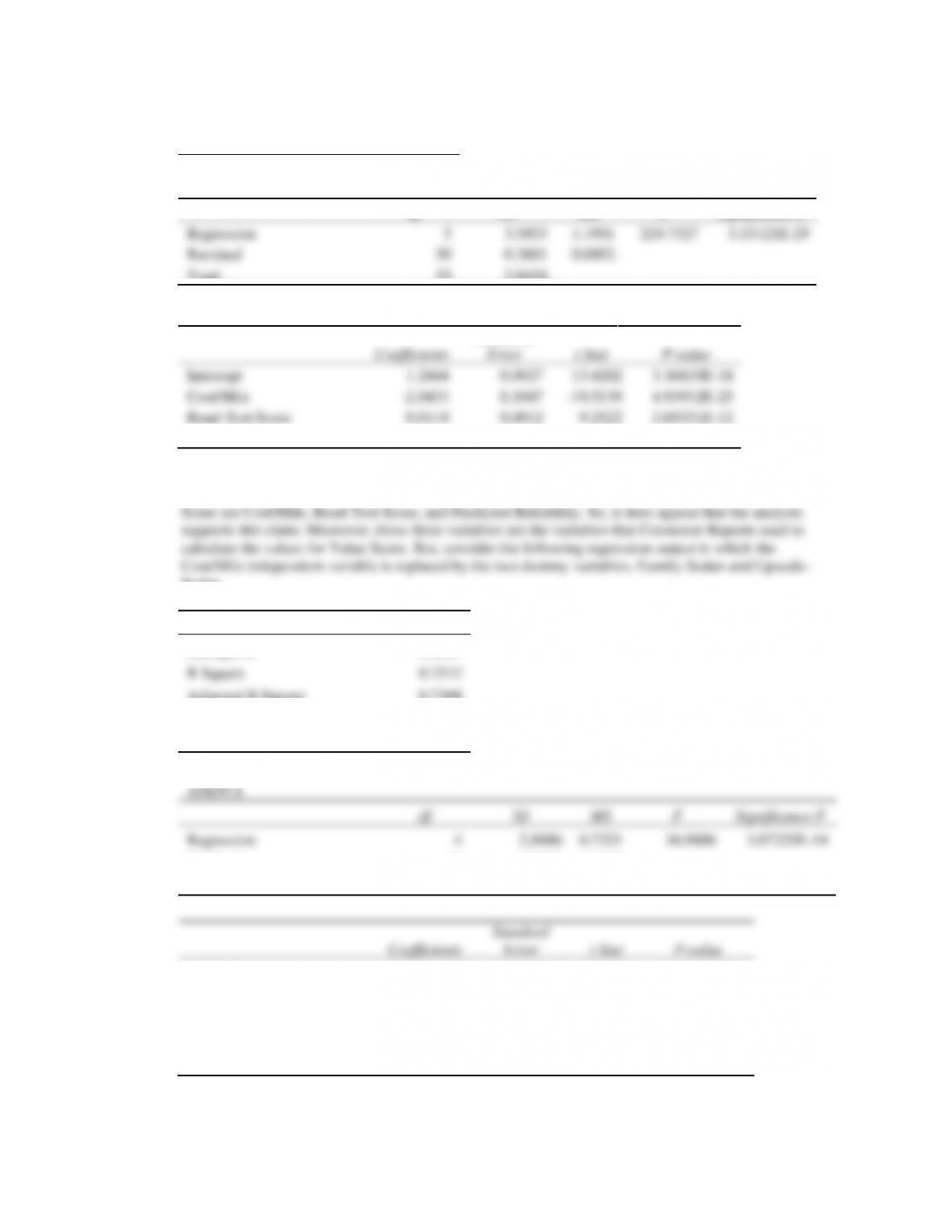
4. The estimated regression equation developed in part (3) shows that the three best predictors of Value
Sedan.
Regression Statistics
Multiple R
0.8667
R Square
0.7512
Adjusted R Square
0.7309
Standard Error
0.1397
Observations
54
ANOVA
df
SS
MS
F
Significance F
Regression
4
2.8886
0.7221
36.9806
3.07225E-14
Residual
49
0.9569
0.0195
Total
53
3.8454
Coefficients
Standard
Error
t Stat
P-value
Intercept
0.1719
0.1840
0.9341
0.3548
Family-Sedan
-0.2499
0.0582
-4.2948
8.24809E-05
Upscale-Sedan
-0.4553
0.0576
-7.9090
2.63274E-10
Road-Test Score
0.0112
0.0025
4.3800
6.23668E-05
Predicted Reliability
0.1701
0.0202
8.4018
4.67372E-11
This regression output shows that the size of the car, as represented by the two dummy variables is
also a significant factor in predicting Value Score. But, note that in part (1) the estimated regression
equation shows that there is a significant relationship between Cost/Mile and the two dummy
variables representing size. So, once the effect of Cost/Mile has been accounted for, any effects that
might be due to size have already been incorporated into the model.