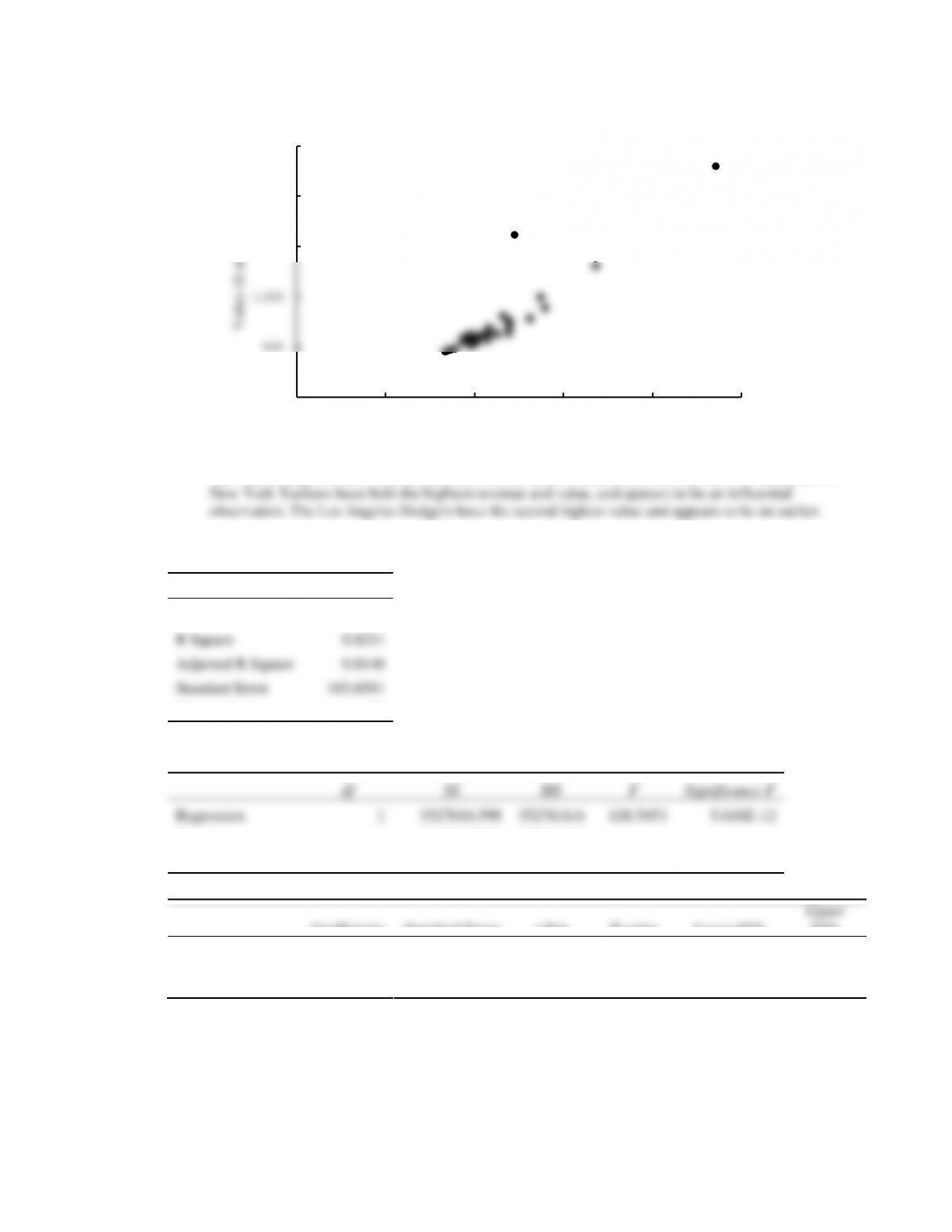
54. a.
The scatter diagram does indicate potential outliers and/or influential observations. For example, the
b. A portion of the Excel output follows:
Regression Statistics
Multiple R
0.9062
R Square
0.8211
Adjusted R Square
0.8148
Standard Error
165.6581
Observations
30
ANOVA
df
SS
MS
F
Significance F
Regression
1
3527616.598
3527616.6
128.5453
5.616E-12
Residual
28
768392.7687
27442.599
Total
29
4296009.367
Coefficients
Standard Error
t Stat
P-value
Lower 95%
Upper
95%
Intercept
-601.4814
122.4288
-4.9129
3.519E-05
-852.2655
-350.6973
Revenue ($
millions)
5.9271
0.5228
11.3378
5.616E-12
4.8562
6.9979
Thus, the estimated regression equation that can be used to predict the team’s value given the value
of annual revenue is
ˆ
y
= -601.4814 + 5.9271 Revenue.
0
500
1,000
1,500
2,000
2,500
0100 200 300 400 500
Value ($ millions)
Revenue ($ millions)
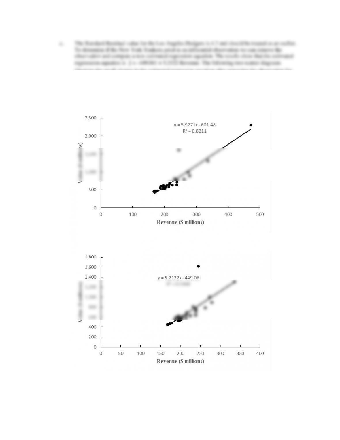
illustrate the small change in the estimated regression equation after removing the observation for
the New York Yankees. These scatter diagrams show that the effect of the New York Yankees
observation on the regression results is not that dramatic.
Scatter Diagram Including the New York Yankees Observation
Scatter Diagram Excluding the New York Yankees Observation
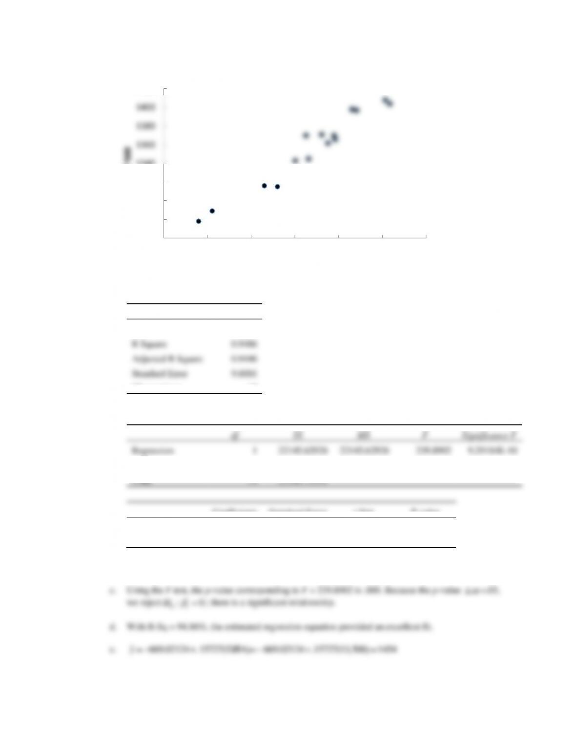
55. a.
b. A portion of the Excel output is shown below:
Regression Statistics
Multiple R
0.9740
R Square
0.9486
Adjusted R Square
0.9446
Standard Error
9.6081
Observations
15
ANOVA
df
SS
MS
F
Significance F
Regression
1
22145.62926
22145.62926
239.8902
9.29184E-10
Residual
13
1200.1041
92.3157
Total
14
23345.73333
Coefficients
Standard Error
t Stat
P-value
Intercept
-669.02124
130.7336
-5.1174
0.0002
DJIA
0.15727
0.0102
15.4884
9.29184E-10
ˆ
y
= -669.02124 + 0.15727 DJIA
1260
1280
1300
1320
1340
1360
1380
1400
1420
12200 12400 12600 12800 13000 13200 13400
S&P 500
DJIA
f. The DJIA is not that far beyond the range of the data. With the excellent fit provided by the
estimated regression equation, we should not be too concerned about using the estimated regression
equation to predict the S&P500.
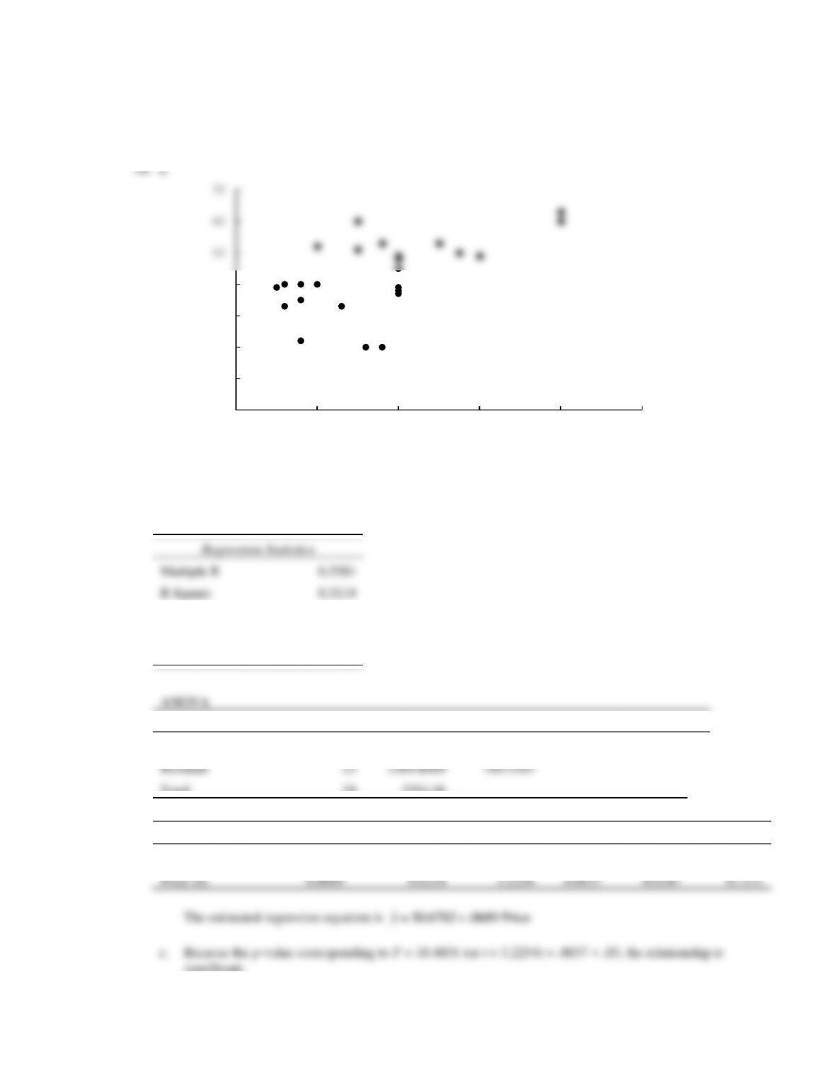
There appears to be a positive linear relationship between the two variables.
b. A portion of the Excel Regression tool output follows:
Regression Statistics
Multiple R
0.5581
R Square
0.3114
Adjusted R Square
0.2815
Standard Error
10.0213
Observations
25
ANOVA
df
SS
MS
F
Significance F
Regression
1
1044.7511
1044.7511
10.4031
0.0037
Residual
23
2309.8089
100.4265
Total
24
3354.56
Coefficients
Standard Error
t Stat
P-value
Lower 95%
Upper 95%
Intercept
30.6782
4.2483
7.2212
2.37E-07
21.8899
39.4666
Price ($)
0.0689
0.0214
3.2254
0.0037
0.0247
0.1131
The estimated regression equation is
ˆ30.6782 .0689 Pricey=+
c. Because the p-value corresponding to F = 10.4031 (or t = 3.2254) = .0037 < .05, the relationship is
significant.
0
10
20
30
40
50
60
70
0100 200 300 400 500
Rating
Price ($)
d. R Square = .3114 indicates that the fit provided by the estimated regression equation is not that
good.
e. Outliers
Observation 12: Klipsch KMC 3
Observation 14: Libratone Zipp
f.
ˆ
y
= 30.6782 + .0689 Price($) = 30.6782 + .0689(400) = 58.24 or approximately 58
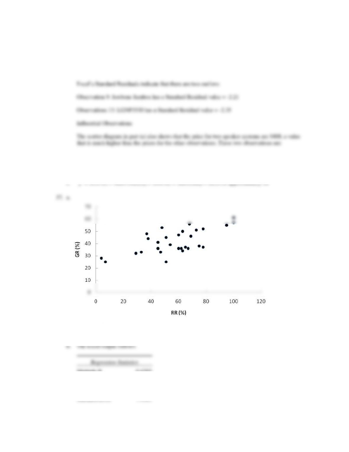
The scatter diagram indicates a positive linear relationship between the two variables. Online
universities with higher retention rates tend to have higher graduation rates.

Observations
29
ANOVA
df
SS
MS
F
Significance F
Regression
1
1224.2860
1224.2860
22.0221
6.95491E-05
Residual
27
1501.0244
55.5935
Total
28
2725.3103
Coefficients
Standard Error
t Stat
P-value
Lower 95%
Upper 95%
Intercept
25.4229
3.7463
6.7862
2.7441E-07
17.7362
33.1096
RR(%)
0.2845
0.0606
4.6928
6.95491E-05
0.1601
0.4089
ˆ
y
= 25.4229 + 0.2845 RR(%)
c. Because the p-value = .000 < α =.05, the relationship is significant.
d. The estimated regression equation is able to explain 44.92% of the variability in the graduation rate
based upon the linear relationship with the retention rate. It is not a great fit, but given the type of
data, the fit is reasonably good.
e. With a retention rate of 51% it does appear that the graduation rate of 25% is low as compared to the
results for other online universities. The president of South University should be concerned after
looking at the data. Using the estimated regression equation, we estimate that the graduation rate at
South University should be 25.4229 + .2845(51) = 40%.
58. The Excel output is shown below:
Regression Statistics
Multiple R
0.9253
R Square
0.8562
Adjusted R Square
0.8382
Standard Error
4.2496
Observations
10
ANOVA
df
SS
MS
F
Significance F
Regression
1
860.0509486
860.0509
47.6238
0.0001
Residual
8
144.4740514
18.0593
Total
9
1004.525

Coefficients
Standard Error
t Stat
P-value
Intercept
10.5280
3.7449
2.8113
0.0228
Weekly Usage
0.9534
0.1382
6.9010
0.0001
a.
ˆ
y
= 10.528 + .9534x
d. Yes, since the expected expense is $3913.
59. a. The Excel output is shown below:
Regression Statistics
Multiple R
0.9341
R Square
0.8725
Adjusted R Square
0.8566
Standard Error
75.4983
Observations
10
ANOVA
df
SS
MS
F
Significance F
Regression
1
312050
312050
54.7456
7.62662E-05
Residual
8
45600
5700
Total
9
357650
Coefficients
Standard Error
t Stat
P-value
Intercept
220
58.4808
3.7619
0.0055
Age
131.6667
17.7951
7.3990
7.63E–05
ˆ
y
= 220 + 131.6667 Age
b. Since the p-value corresponding to F = 54.75 is .000 <
= .05, we reject H0:
1 = 0.
60. A portion of the Excel Regression tool output for this problem follows.
Regression Statistics
Multiple R
0.6852
R Square
0.4695
Adjusted R Square
0.4032
Standard Error
2.6641
Observations
10
ANOVA
df
SS
MS
F
Significance F
Regression
1
50.2554
50.2554
7.0807
0.0288
Residual
8
56.7806
7.0976
Total
9
107.036
Coefficients
Standard Error
t Stat
P-value
Intercept
0.2747
0.9004
0.3051
0.7681
S&P 500
0.9498
0.3569
2.6609
0.0288
a.
ˆ
y
= 0.2747 + 0.9498 S&P 500 Market beta = .95
61. a.
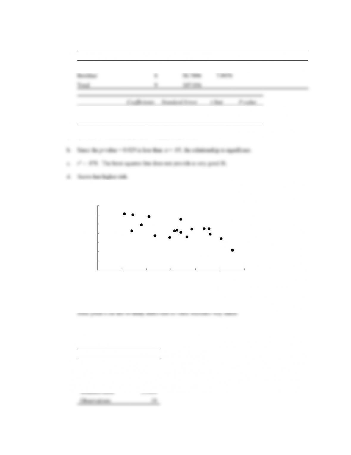
b. There appears to be a negative relationship between the two variables that can be approximated by a
straight line. An argument could also be made that the relationship is perhaps curvilinear because at
c. The Excel output is shown below.
Regression Statistics
Multiple R
0.7339
R Square
0.5387
Adjusted R Square
0.5115
Standard Error
1.5414
Observations
19
4.0
6.0
8.0
10.0
12.0
14.0
16.0
18.0
020 40 60 80 100 120
Price ($1000s)
Miles (1000s)
ANOVA
df
SS
MS
F
Significance F
Regression
1
47.1580
47.1580
19.8490
0.0003
Residual
17
40.3893
2.3758
Total
18
87.5474
Coefficients
Standard Error
t Stat
P-value
Intercept
16.4698
0.9488
17.3592
2.98677E-12
Miles (1000s)
-0.0588
0.0132
-4.4552
0.0003
ˆ
y
= 16.4698 – 0.0588 Miles (1000s)
d. Significant relationship: p-value = 0.000 < α = .05.
e.
2
r
= .5387; a reasonably good fit considering that the condition of the car is also an important factor
in what the price is.
f. The slope of the estimated regression equation is -.0558. Thus, a one-unit increase in the value of x
coincides with a decrease in the value of y equal to .0558. Because the data were recorded in
thousands, every additional 1000 miles on the car’s odometer will result in a $55.80 decrease in the
62. a.
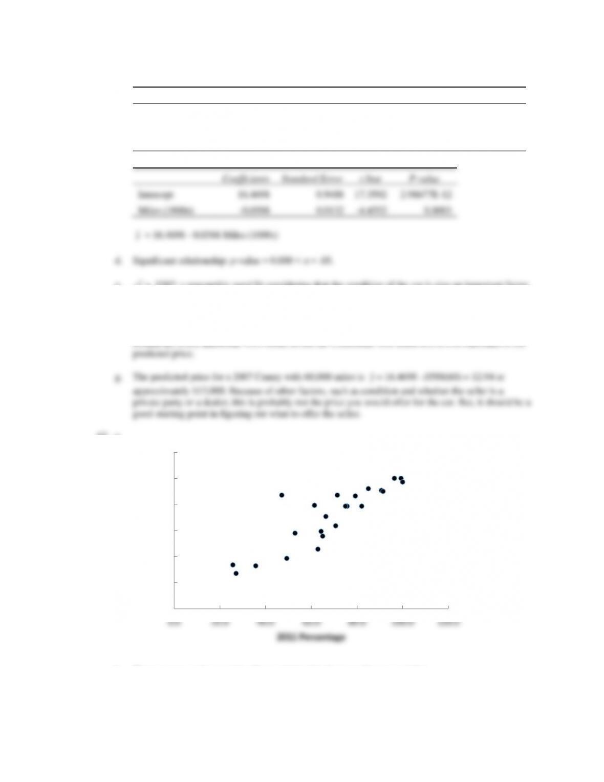
b. There appears to be a positive linear relationship between the two variables.
c. The Excel output is shown below.
0.0
20.0
40.0
60.0
80.0
100.0
120.0
0.0 20.0 40.0 60.0 80.0 100.0 120.0
2012 Percentage
2011 Percentage

Regression Statistics
Multiple R
0.8702
R Square
0.7572
Adjusted R Square
0.7456
Standard Error
11.5916
Observations
23
ANOVA
df
SS
MS
F
Significance F
Regression
1
8798.2391
8798.2391
65.4802
6.85277E-08
Residual
21
2821.6609
134.3648
Total
22
11619.9
Coefficients
Standard Error
t Stat
P-value
Intercept
7.3880
8.2125
0.8996
0.3785
2011 Percentage
0.9276
0.1146
8.0920
6.85277E-08
e.
2
r
= .7572; a good fit.
f.
The point with a residual value of approximately 36 clearly stands out as compared to the other
points. This point corresponds to the observation for Air Tran Airways. Other than this point, the
residual plot does not exhibit a pattern that would suggest a linear model is not appropriate.
-30
-20
-10
0
10
20
30
40
0.0 20.0 40.0 60.0 80.0 100.0 120.0
Residuals
2011 Percentage