10. a.
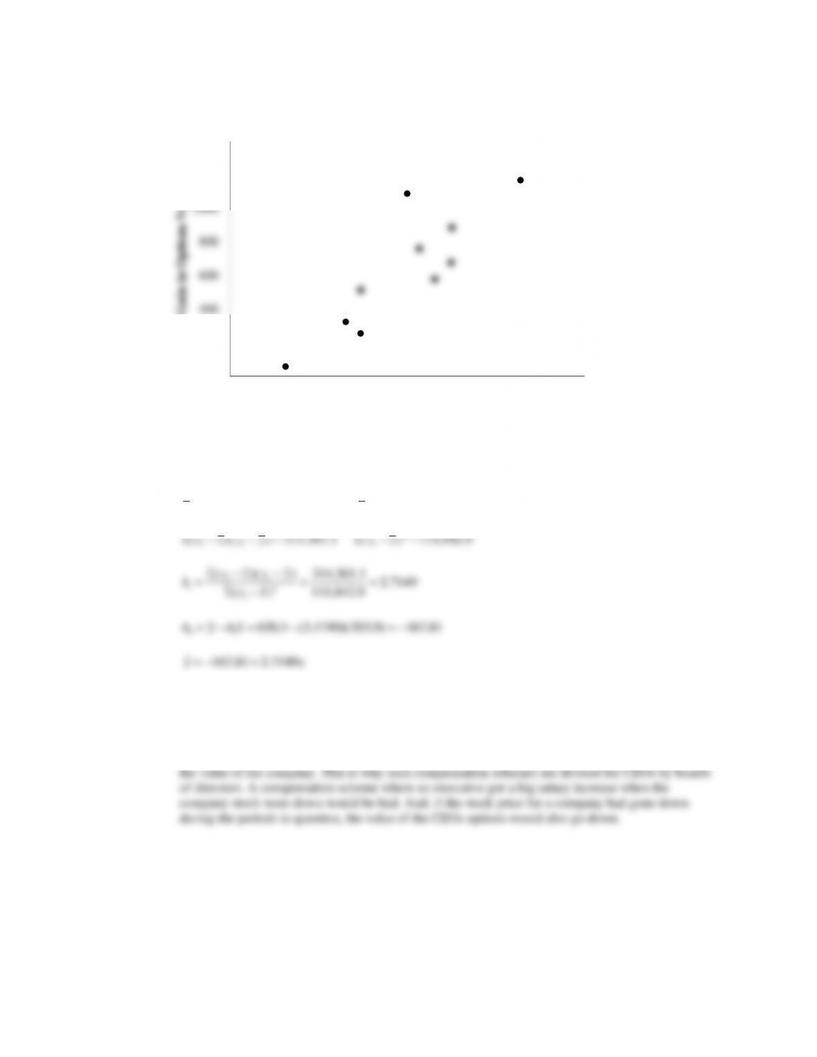
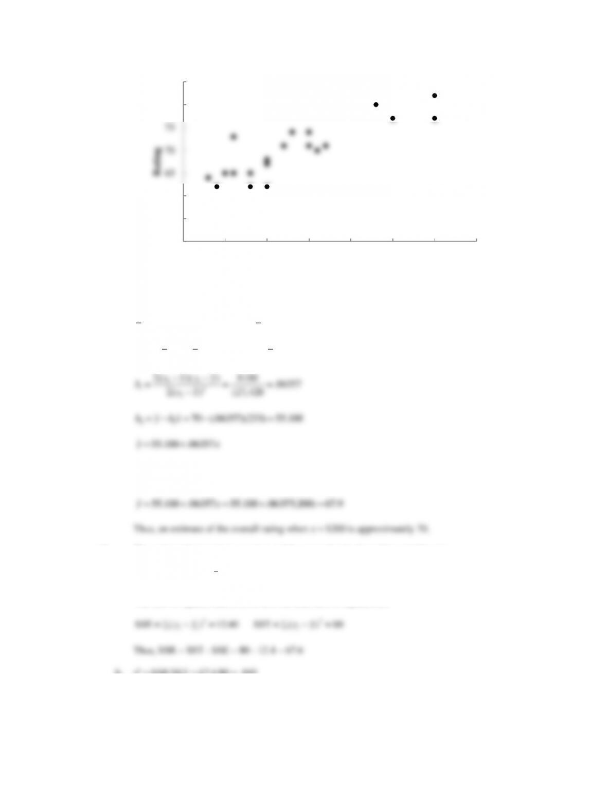
b. The scatter diagram indicates a positive linear relationship between x = percentage increase in the
stock price and y = percentage gain in options value. In other words, options values increase as stock
prices increase.
c.
/ 2939/10 293.9 / 6301/10 630.1
ii
x x n y y n= = = = = =
2
12
( )( ) 314,501.1 2.7149
( ) 115,842.9
ii
i
x x y y
bxx
− −
= = =
−
01
630.1 (2.1749)(293.9) 167.81b y bx= − = − = −
ˆ167.81 2.7149yx= − +
d. The slope of the estimated regression line is approximately 2.7. So, for every percentage increase in
the price of the stock the options value increases by 2.7%.
e. The rewards for the CEO do appear to be based upon performance increases in the stock value.
While the rewards may seem excessive, the executive is being rewarded for his/her role in increasing
0
200
400
600
800
1000
1200
1400
0 100 200 300 400 500 600
% Gain in Options Value
% Increase in Stock Price
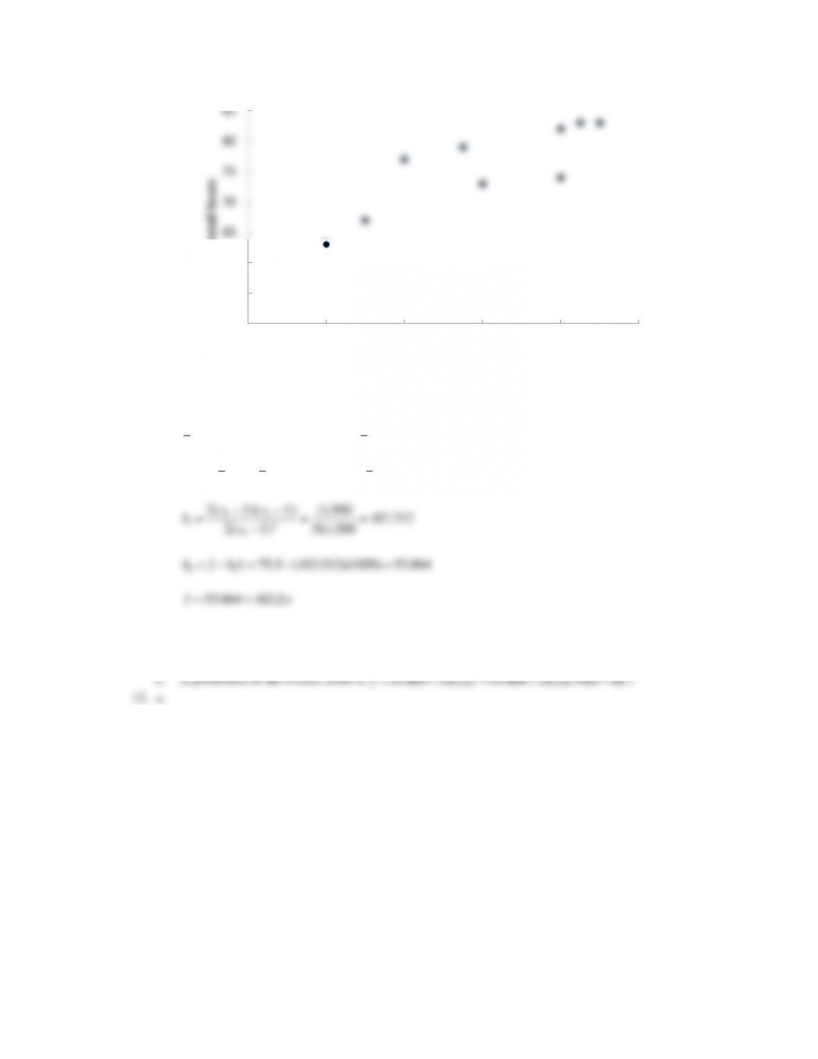
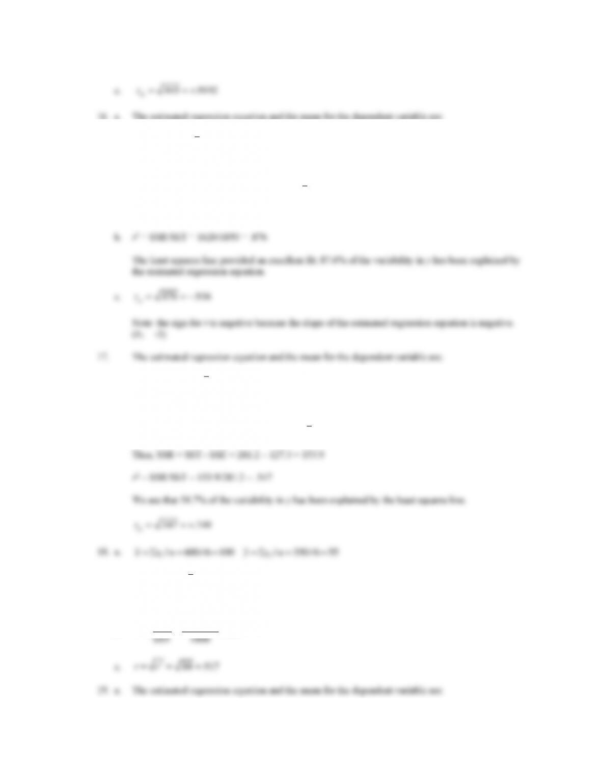
b. The scatter diagram indicates a positive linear relationship between x = price ($) and y = overall
score.
c.
/ 10,200/10 1020 / 755/10 75.5
ii
x x n y y n= = = = = =
2
( )( ) 11,900 ( ) 561,000
i i i
x x y y x x − − = − =
d. The slope of .0212 means that spending an additional $100 in price will increase the overall score by
approximately 2 points.
50
55
60
65
70
75
80
85
400 600 800 1000 1200 1400
Overall Score
Price ($)
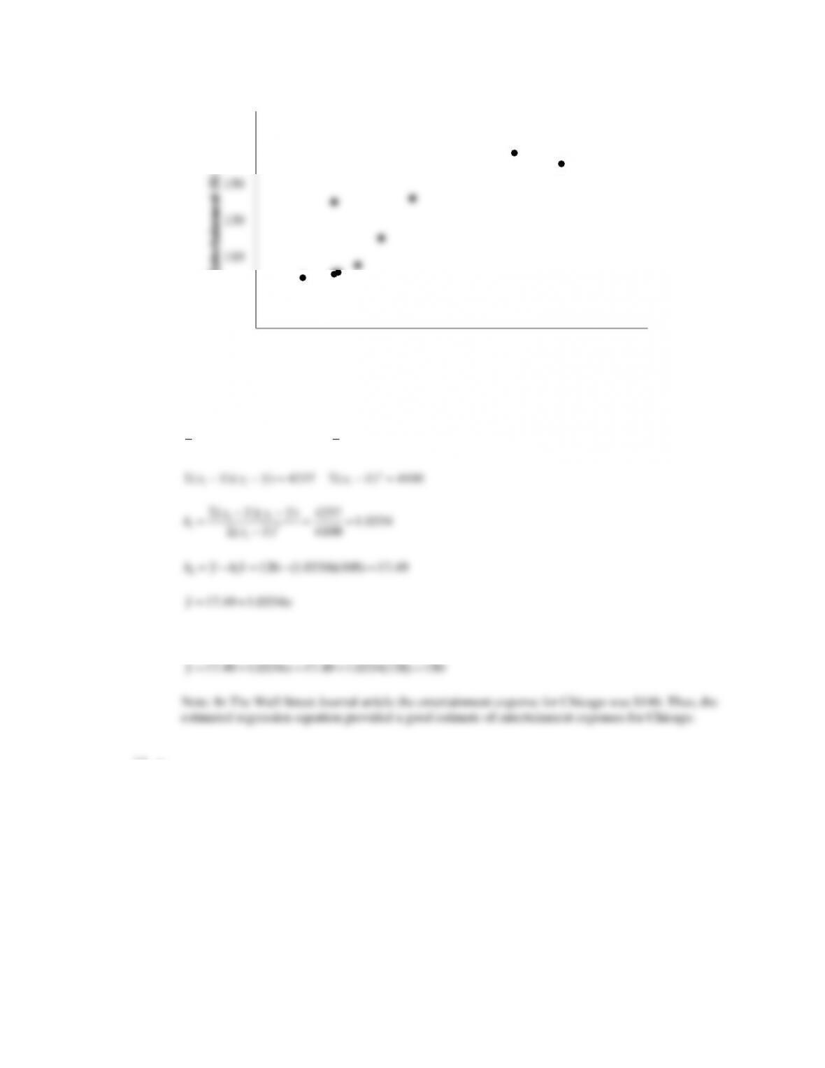
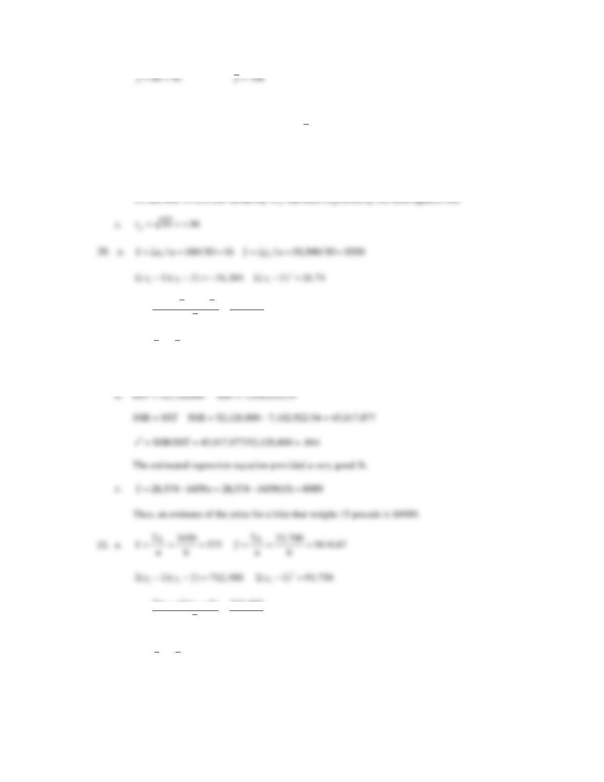
b. The scatter diagram indicates a positive linear relationship between x = hotel room rate and the
amount spent on entertainment.
c.
/ 945/9 105 / 1134/9 126
ii
x x n y y n= = = = = =
d. With a value of x = $128, the predicted value of y for Chicago is
13. a.
70
90
110
130
150
170
190
70 90 110 130 150 170
Entertainment ($)
Hotel Room Rate ($)
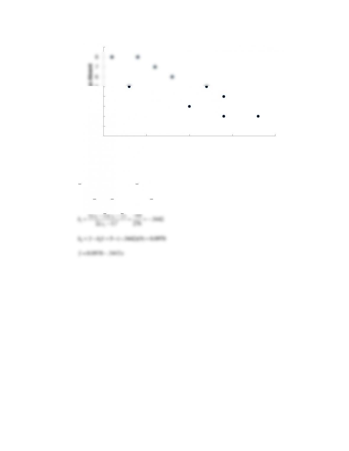
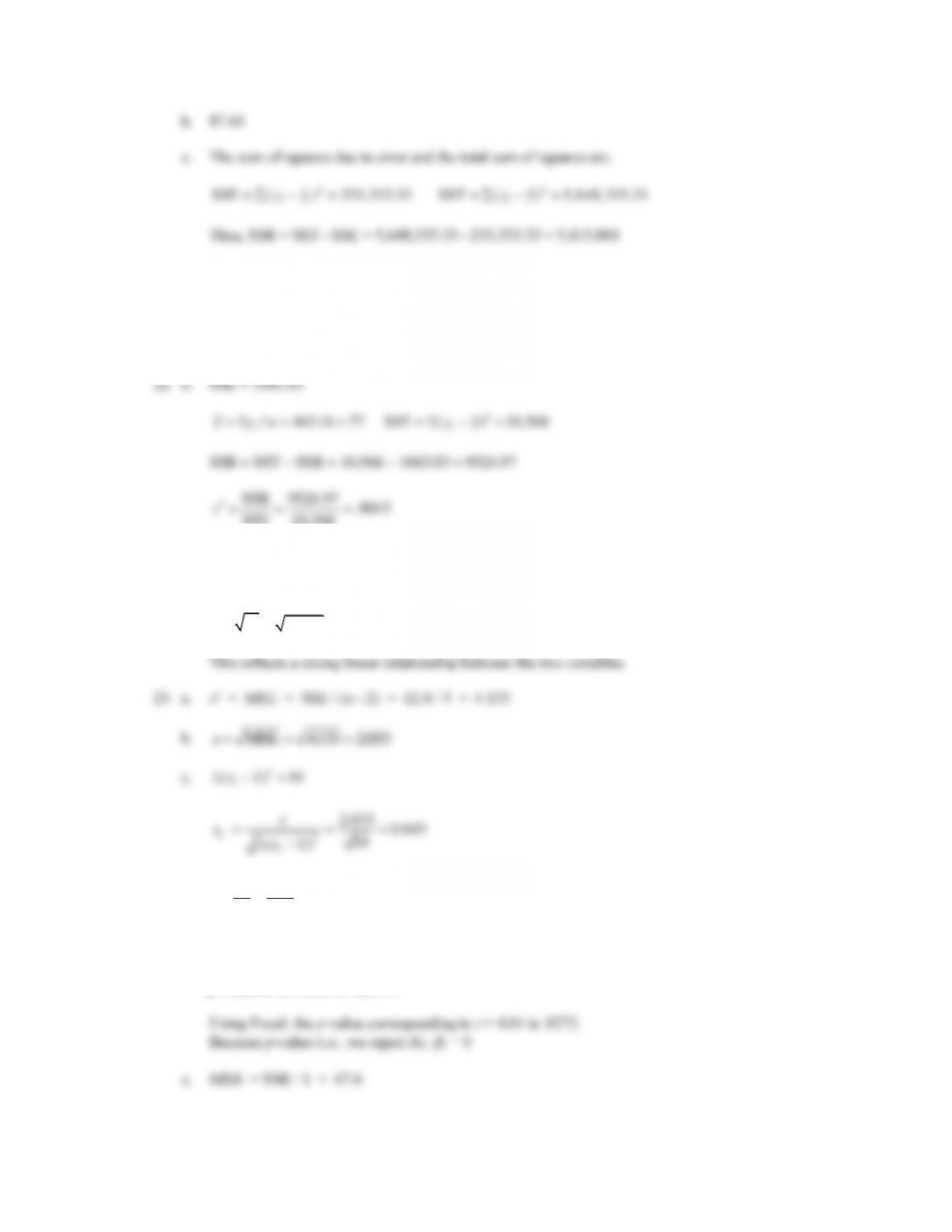
The scatter diagram indicates a negative linear relationship between x = distance to work and y =
number of days absent.
b.
/ 90/10 9 / 50/10 5
ii
x x n y y n= = = = = =
2
( )( ) 95 ( ) 276
i i i
x x y y x x − − = − − =
( )( ) 95 .3442
ii
x x y y
− − −
c. A prediction of the number of days absent is
ˆ8.0978 .3442(5) 6.4y= − =
or approximately 6 days.
14. a.
0
1
2
3
4
5
6
7
8
9
0 5 10 15 20
Number of Days Absent
Distance to Work (miles)
b. The scatter diagram indicates a positive linear relationship between x = price ($) and y = overall
rating.
c.
/ 4660/20 233 / 1400/20 70
ii
x x n y y n= = = = = =
2
( )( ) 8100 ( ) 127,420
i i i
x x y y x x − − = − =
( )( ) 8100 .06357
ii
x x y y
− −
d. We can use the estimated regression equation developed in part (c) to estimate the overall
satisfaction rating corresponding to x = 200.
15. a. The estimated regression equation and the mean for the dependent variable are:
. .y x y
i i
= + =02 26 8
The sum of squares due to error and the total sum of squares are
The least squares line provided a very good fit; 84.5% of the variability in y has been explained by
the least squares line.
50
55
60
65
70
75
80
85
100 150 200 250 300 350 400 450
Rating
Price ($)
16. a. The estimated regression equation and the mean for the dependent variable are:
ˆ68 3 35
i
y x y= − =
The sum of squares due to error and the total sum of squares are
22
ˆ
SSE ( ) 230 SST ( ) 1850
i i i
y y y y= − = = − =
Thus, SSR = SST – SSE = 1850 – 230 = 1620
ˆ7.6 .9 16.6
i
y x y= + =
The sum of squares due to error and the total sum of squares are
22
ˆ
SSE ( ) 127.3 SST ( ) 281.2
i i i
y y y y= − = = − =
22
ˆ
SST = ( ) 1800 SSE = ( ) 287.624
i i i
y y y y − = − =
SSR = SST – SSR = 1800 – 287.624 = 1512.376
b.
2SSR 1512.376 .84
SST 1800
= = =r
The sum of squares due to error and the total sum of squares are
22
ˆ
SSE ( ) 170 SST ( ) 2442
i i i
y y y y= − = = − =
Thus, SSR = SST – SSE = 2442 – 170 = 2272
b. r2 = SSR/SST = 2272/2442 = .93
12
( )( ) 31,284 1439
( ) 21.74
ii
i
x x y y
bxx
− − −
= = = −
−
01
5550 ( 1439)(16) 28,574b y b x= − = − − =
ˆ28,574 1439yx=−
12
( )( ) 712,500 7.6
93,750
()
ii
i
x x y y
bxx
− −
= = =
−
01
5616.67 (7.6)(575) 1246.67b y b x= − = − =
. .y x= +124667 76
r2 = SSR/SST = 5,415,000/5,648,333.33 = .9587
We see that 95.87% of the variability in y has been explained by the estimated regression equation.
d.
. . . . (500) $5046.y x= + = + =124667 76 1246 67 76 67
Source
of Variation
Sum
of Squares
Degrees
of Freedom
Mean
Square
F
p-value
Regression
67.6
1
67.6
16.36
.0272
Error
12.4
3
4.133
Total
80.0
4
b.
MSE 76.6667 8.7560s= = =
c.
2
( ) 180
i
xx − =
12
8.7560 0.6526
180
()
b
i
s
−
d.
1
134.59
.653
b
b
ts
−
= = = −
Using t table (3 degrees of freedom), area in tail is less than .01; p-value is less than .02
Using Excel, the p-value corresponding to t = -4.59 is .0193.
Source
of Variation
Sum
of Squares
Degrees
of Freedom
Mean
Square
F
p-value
Regression
1620
1
1620
21.13
.0193
Error
230
3
76.6667
Total
1850
4
b.
2
( ) 190
i
xx − =
6.5141 0.4726
s
c.
Source
of Variation
Sum
of Squares
Degrees
of Freedom
Mean
Square
F
p-value
Regression
1512.376
1
1512.376
21.03
.010
Error
287.624
4
71.906
Total
1800
5