
Chapter 12
Simple Linear Regression
Learning Objectives
1. Understand how regression analysis can be used to develop an equation that estimates
mathematically how two variables are related.
2. Understand the differences between the regression model, the regression equation, and the estimated
regression equation.
3. Know how to fit an estimated regression equation to a set of sample data based upon the least–
squares method.
4. Be able to determine how good a fit is provided by the estimated regression equation and compute
the sample correlation coefficient from the regression analysis output.
5. Understand the assumptions necessary for statistical inference and be able to test for a significant
relationship.
6. Know how to develop confidence interval estimates of y given a specific value of x in both the case
of a mean value of y and an individual value of y.
7. Learn how to use a residual plot to make a judgement as to the validity of the regression
assumptions.
8. Know the definition of the following terms:
independent and dependent variable
simple linear regression
regression model
regression equation and estimated regression equation
scatter diagram
coefficient of determination
standard error of the estimate
confidence interval
prediction interval
residual plot
Solutions:
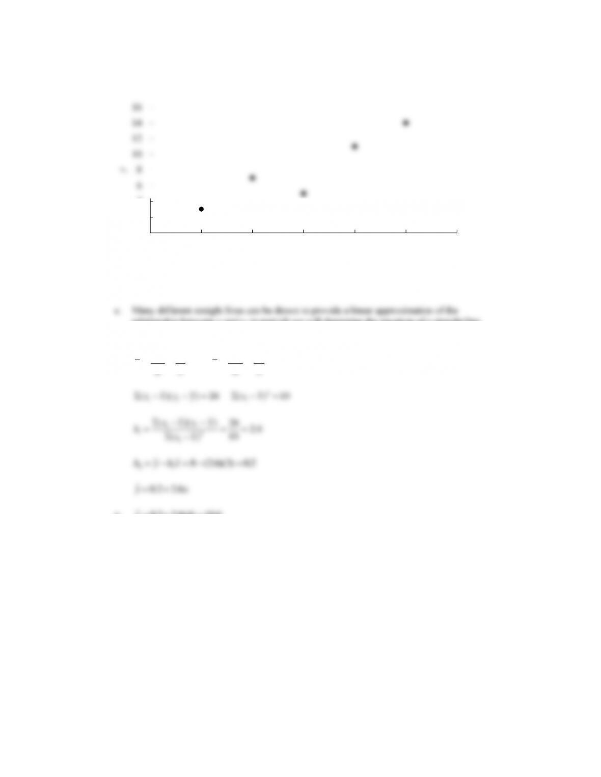
1 a.
b. There appears to be a positive linear relationship between x and y.
relationship between x and y; in part (d) we will determine the equation of a straight line
that “best” represents the relationship according to the least squares criterion.
d.
15 40
3 8
55
ii
xy
xy
nn
= = = = = =
e.
ˆ0.2 2.6(4) 10.6y= + =
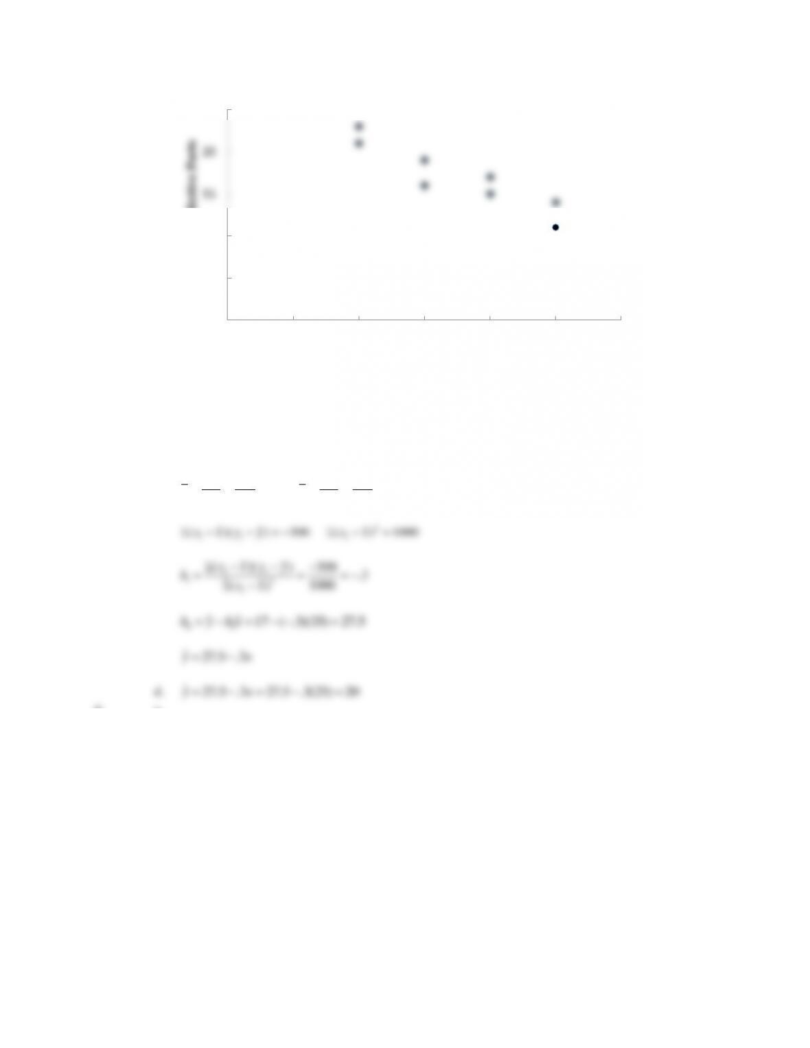
2. a.
0
2
4
6
8
10
12
14
16
0123456
y
x
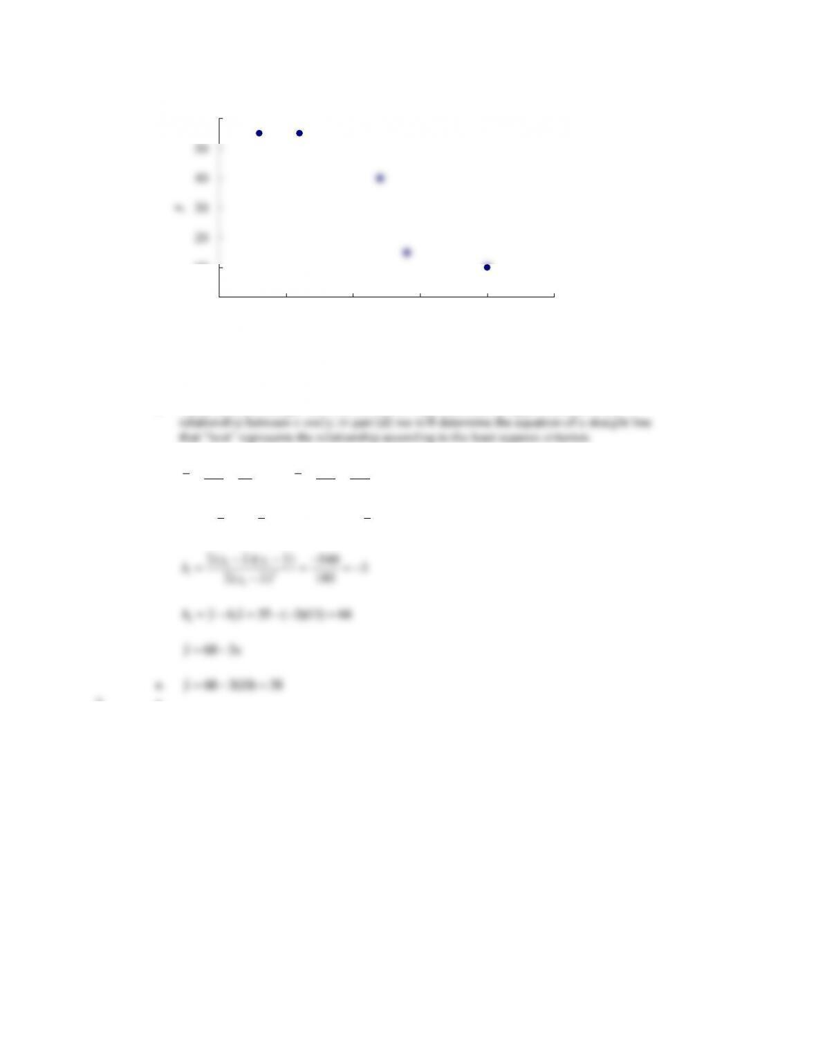
b. There appears to be a negative linear relationship between x and y.
c. Many different straight lines can be drawn to provide a linear approximation of the
d.
55 175
11 35
55
ii
xy
xy
nn
= = = = = =
2
( )( ) 540 ( ) 180
i i i
x x y y x x − − = − − =
( )( ) 540 3
ii
x x y y
− − −
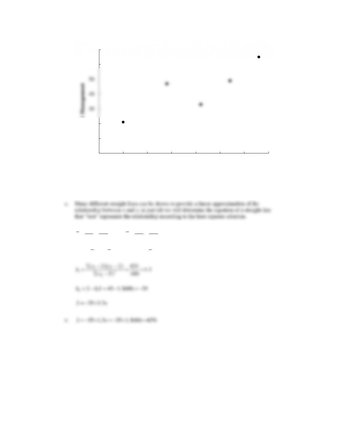
3. a.
0
10
20
30
40
50
60
0 5 10 15 20 25
y
x
b.
50 83
10 16.6
55
ii
xy
xy
nn
= = = = = =
2
( )( ) 171 ( ) 190
i i i
x x y y x x − − = − =
( )( ) 171 0.9
ii
x x y y
− −
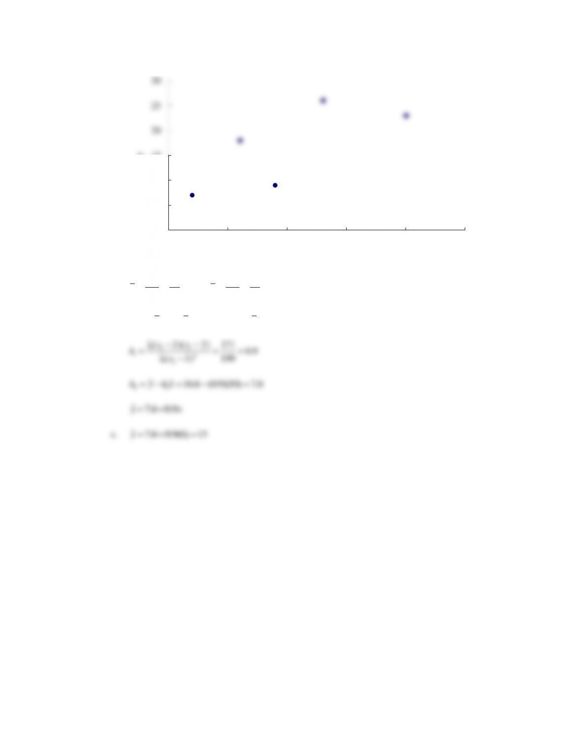
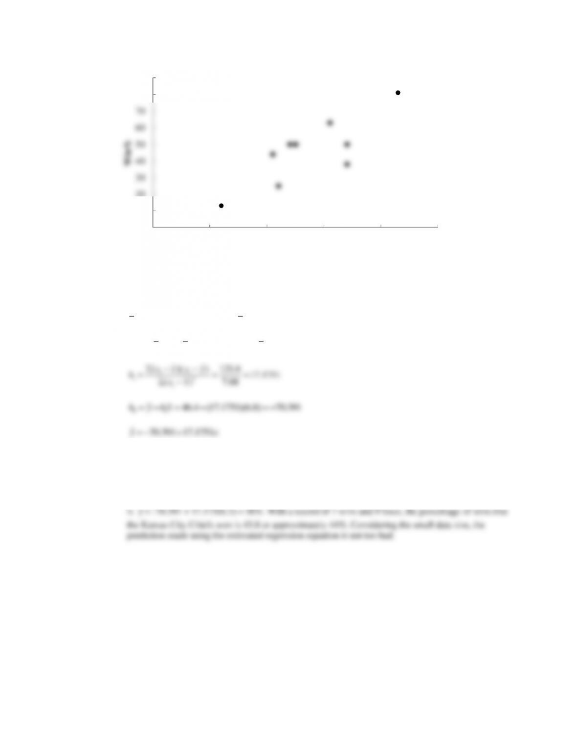
4. a.
0
5
10
15
20
25
30
0 5 10 15 20 25
y
x
b. There appears to be a positive linear relationship between the percentage of women working in the
five companies (x) and the percentage of management jobs held by women in that company (y)
d.
300 215
60 43
55
ii
xy
xy
nn
= = = = = =
2
( )( ) 624 ( ) 480
i i i
x x y y x x − − = − =
( )( ) 624 1.3
ii
x x y y
− −
5. a.
0
10
20
30
40
50
60
70
40 45 50 55 60 65 70 75
% Management
% Working
b. There appears to be a negative relationship between line speed (feet per minute) and the number of
defective parts.
c. Let x = line speed (feet per minute) and y = number of defective parts.
280 136
35 17
88
ii
xy
xy
nn
= = = = = =
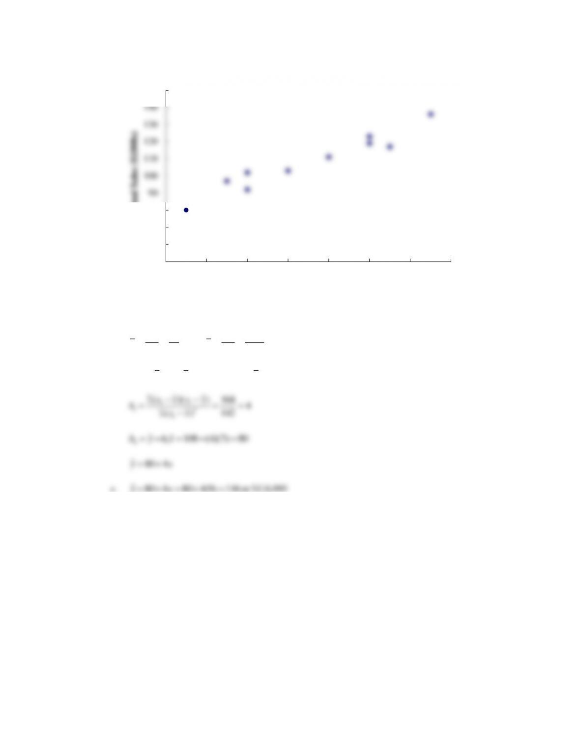
6. a.
0
5
10
15
20
25
010 20 30 40 50 60
Number of Defective Parts
Line Speed (feet per minute)
b. The scatter diagram indicates a positive linear relationship between x = average number of passing
yards per attempt and y = the percentage of games won by the team.
c.
/ 680/10 6.8 / 464/10 46.4
ii
x x n y y n= = = = = =
2
( )( ) 121.6 ( ) 7.08
i i i
x x y y x x − − = − =
d. The slope of the estimated regression line is approximately 17.2. So, for every increase of one yard
in the average number of passes per attempt, the percentage of games won by the team increases by
17.2%.
e. With an average number of passing yards per attempt of 6.2, the predicted percentage of games won
7. a.
0
10
20
30
40
50
60
70
80
90
4 5 6 7 8 9
Win%
Yds/Att
b. Let x = years of experience and y = annual sales ($1000s)
70 1080
7 108
10 10
ii
xy
xy
nn
= = = = = =
2
( )( ) 568 ( ) 142
i i i
x x y y x x − − = − =
8. a.
50
60
70
80
90
100
110
120
130
140
150
0 2 4 6 8 10 12 14
Annual Sales ($1000s)
Years of Experience
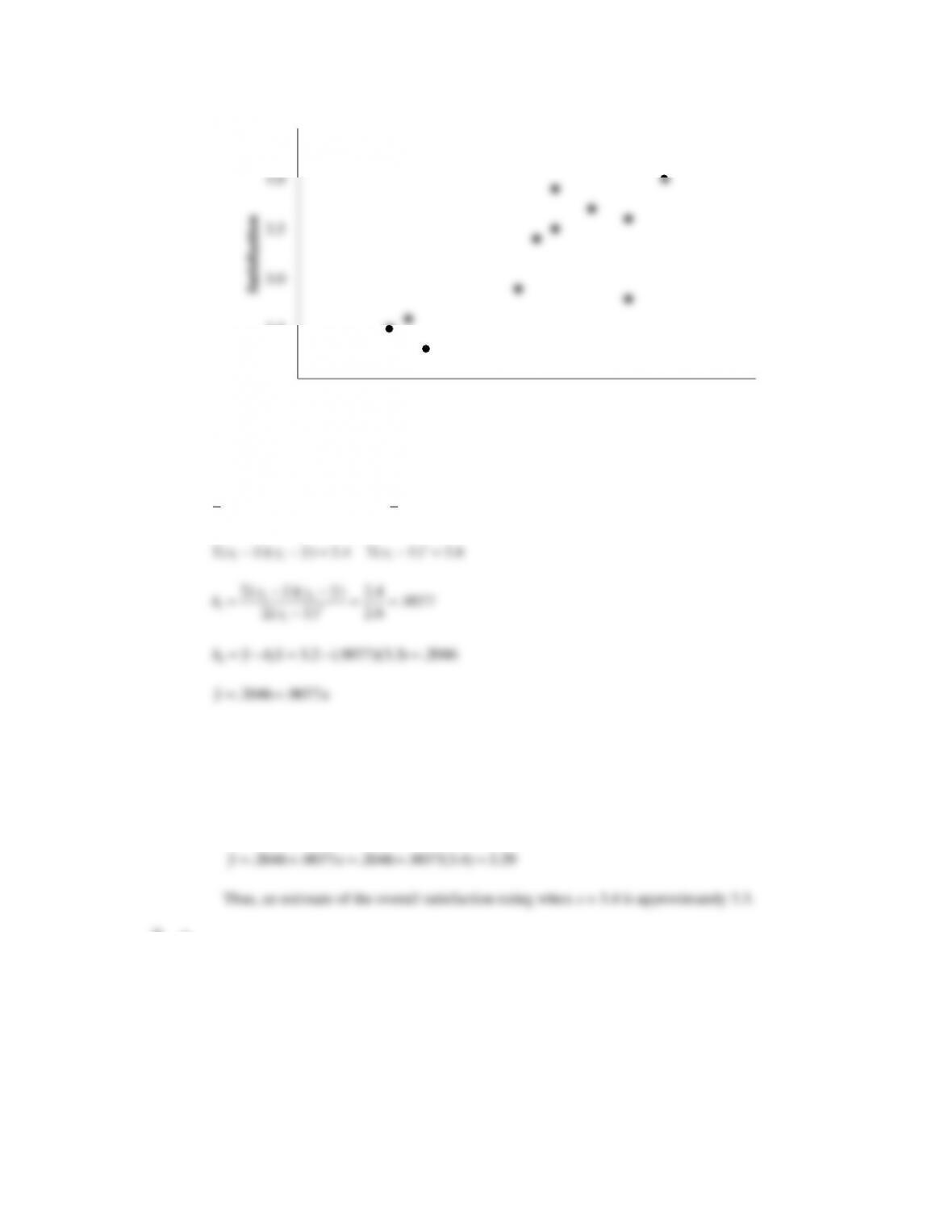
b. The scatter diagram indicates a positive linear relationship between x = speed of execution rating and
y = overall satisfaction rating for electronic trades.
c.
/ 36.3/11 3.3 / 35.2/11 3.2
ii
x x n y y n= = = = = =
2
d. The slope of the estimated regression line is approximately .9077. So, a one unit increase in the
speed of execution rating will increase the overall satisfaction rating by approximately .9 points.
e. The average speed of execution rating for the other brokerage firms is 3.4. Using this as the new
value of x for Zecco.com, we can use the estimated regression equation developed in part (c) to
estimate the overall satisfaction rating corresponding to x = 3.4.
2.0
2.5
3.0
3.5
4.0
4.5
2.0 2.5 3.0 3.5 4.0 4.5
Satisfaction
Speed of Execution
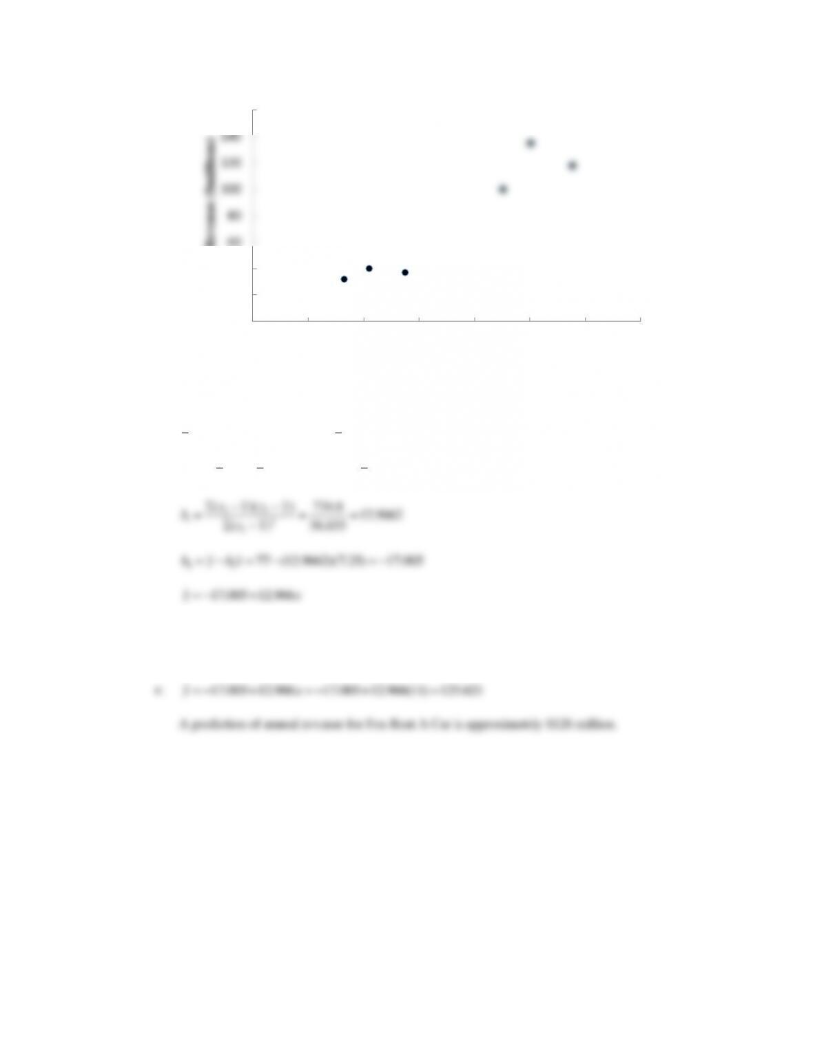
b. The scatter diagram indicates a positive linear relationship between x = cars in service (1000s) and y
= annual revenue ($millions).
c.
/ 43.5/6 7.25 / 462/6 77
ii
x x n y y n= = = = = =
2
( )( ) 734.6 ( ) 56.655
i i i
x x y y x x − − = − =
d. For every additional 1000 cars placed in service annual revenue will increase by 12.966 ($millions)
or $12,966,000. Therefor every additional car placed in service will increase annual revenue by
$12,966.
0
20
40
60
80
100
120
140
160
0246810 12 14
Annual Revenue ($millions)
Cars in Service (1000s)