Chapter 12
Simple Linear Regression
Case Problem 1: Measuring Stock Market Risk
a. Selected descriptive statistics follow:
Variable
N
Mean
StDev
Minimum
Median
Maximum
Microsoft
36
0.00503
0.04537
-0.08201
0.00400
0.08883
Exxon Mobil
36
0.01664
0.05534
-0.11646
0.01279
0.23217
Caterpillar
36
0.03010
0.06860
-0.10060
0.04080
0.21850
Johnson & Johnson
36
0.00530
0.03487
-0.05917
-0.00148
0.10334
McDonald’s
36
0.02450
0.06810
-0.11440
0.03700
0.18260
Sandisk
36
0.06930
0.19540
-0.28330
0.07410
0.50170
Qualcomm
36
0.02840
0.08620
-0.12170
0.03870
0.21060
Procter & Gamble
36
0.01059
0.03707
-0.05365
0.01333
0.08783
S&P 500
36
0.01010
0.02633
-0.03429
0.01034
0.08104
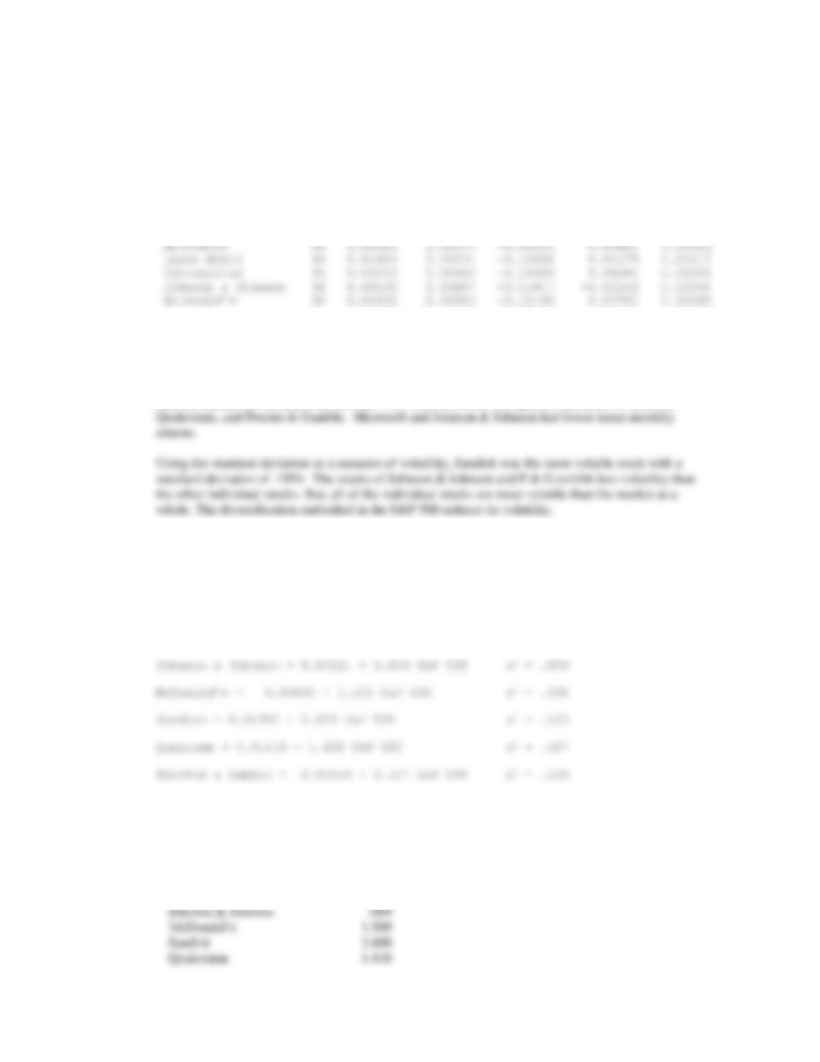
From the descriptive statistics we see that six of the companies had a higher mean monthly return
than the market (as measured by the S&P 500): Exxon Mobil, Caterpillar, McDonald’s, Sandisk,
b. The estimated regression equation relating each of the individual stocks to the S&P 500 is shown
below. The value of r2 for each equation is also shown.
Microsoft = 0.00040 + 0.458 S&P 500 r2 = .071
Exxon Mobil = 0.00926 + 0.731 S&P 500 r2 = .121
Caterpillar = 0.015000 + 1.49 S&P 500 r2 = .329
The betas (slope of estimated regression equation) for the individual stocks can be obtained from the
regression output.
Company Beta
Microsoft .458
Exxon Mobil .731
Caterpillar 1.490
The beta for the market as a whole is 1. So, any stock with a beta greater than 1 will move up faster
c. The r2 values seem to indicate that from 0% to 33.8% of the variability of the returns in these
individual stocks is explained by the return for the market.
Case Problem 2: U.S. Department of Transportation
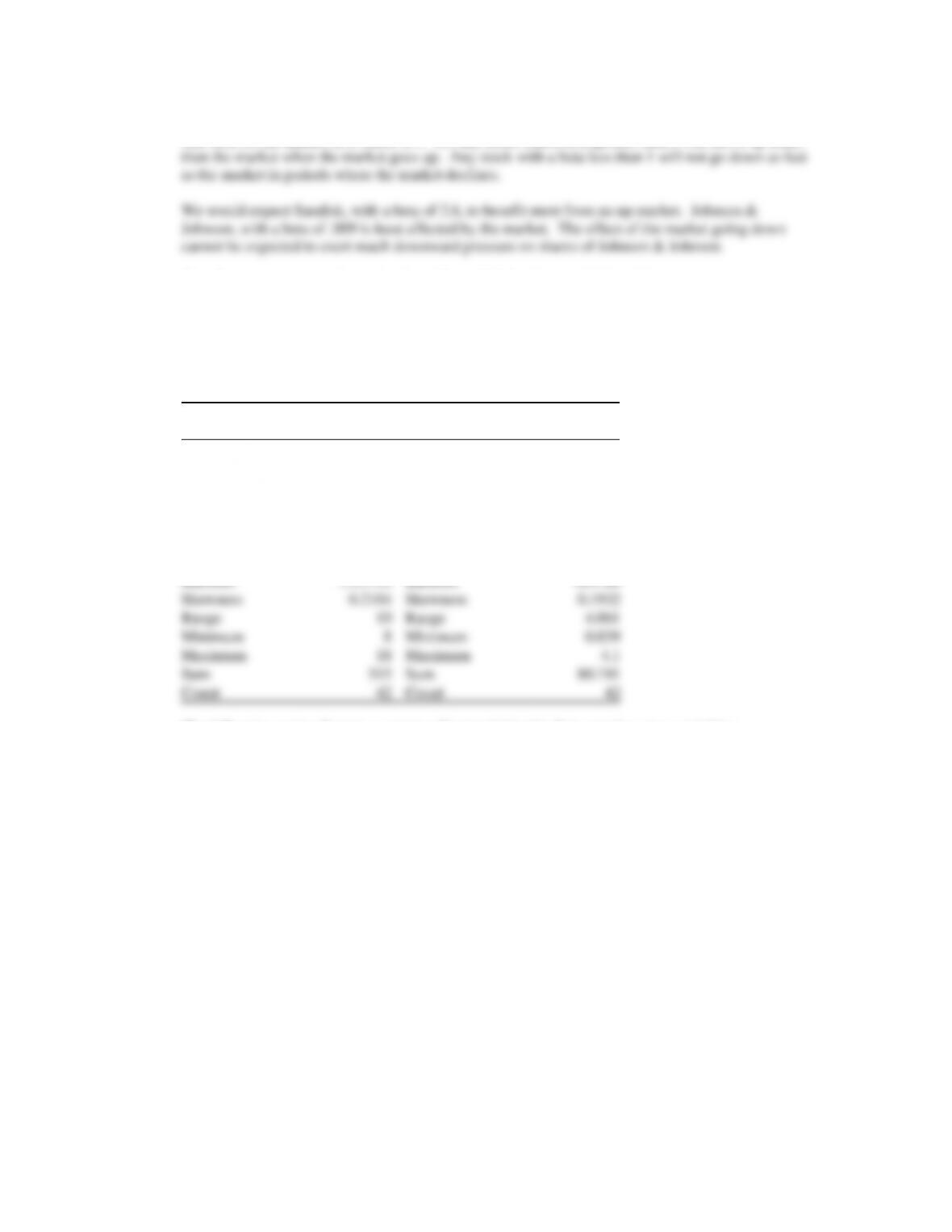
1. The descriptive statistics and graphical summaries are shown below:
Percent
Under 21
Fatal Accidents
per 1000
Mean
12.2619
Mean
1.9224
Standard Error
0.4832
Standard Error
0.1653
Median
12
Median
1.881
Mode
8
Mode
#N/A
Standard Deviation
3.1317
Standard Deviation
1.0710
Sample Variance
9.8078
Sample Variance
1.1470
Kurtosis
-1.13711
Kurtosis
-0.9749
Skewness
0.2104
Skewness
0.1932
Range
10
Range
4.061
Minimum
8
Minimum
0.039
Maximum
18
Maximum
4.1
Sum
515
Sum
80.741
Count
42
Count
42
The following scatter diagram suggests a linear relationship between these two variables:
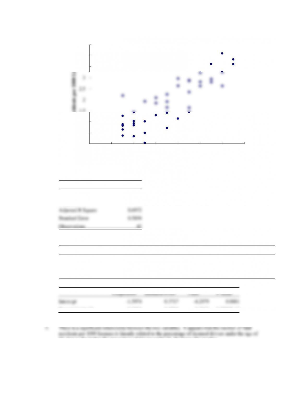
2. A portion of the Excel Regression tool output is shown below:
Regression Statistics
Multiple R
0.8394
R Square
0.7046
Adjusted R Square
0.6972
Standard Error
0.5894
Observations
42
ANOVA
df
SS
MS
F
Significance F
Regression
1
33.1344
33.1344
95.3965
3.79357E-12
Residual
40
13.8934
0.3473
Total
41
47.0278
Coefficients
Standard Error
t Stat
P-value
Intercept
-1.5974
0.3717
-4.2979
0.0001
Percent Under 21
0.2871
0.0294
9.7671
3.7936E–12
21; that is, the higher the percentage of drivers under 21, the larger the number.
Case Problem 3: Selecting a Point and Shoot Digital Camera
0
0.5
1
1.5
2
2.5
3
3.5
4
4.5
5 7 9 11 13 15 17 19
Fatal Accidents per 1000 Licenses
Percent Under 21
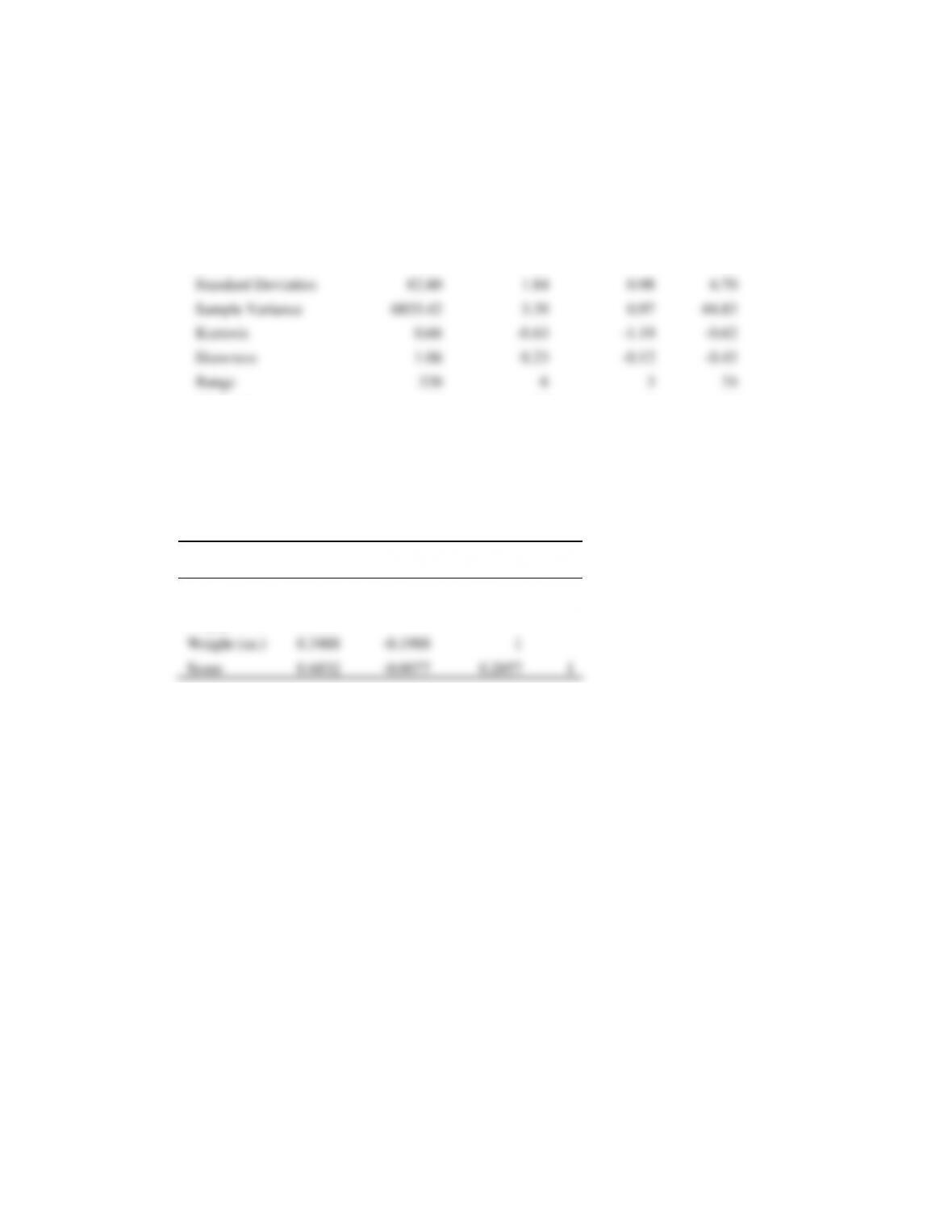
1. Descriptive statistics for the data set follow.
Price ($)
Megapixels
Weight (oz.)
Score
Mean
175.36
12.86
5.82
56.36
Standard Error
15.65
0.35
0.19
1.27
Median
160
12
6
56.5
Mode
200
12
5
66
Standard Deviation
82.80
1.84
0.98
6.70
Sample Variance
6855.42
3.39
0.97
44.83
Kurtosis
0.66
-0.63
-1.19
-0.62
Skewness
1.06
0.23
-0.12
-0.43
Range
320
6
3
24
Minimum
80
10
4
42
Maximum
400
16
7
66
Sum
4910
360
163
1578
Count
28
28
28
28
The sample correlation coefficients for this data set follow.
Price
($)
Megapixels
Weight
(oz.)
Score
Price ($)
1
Megapixels
0.1389
1
Weight (oz.)
0.3488
-0.1988
1
Score
0.6832
-0.0077
0.2857
1
With a sample correlation coefficient of .6832, price appears to be the best predictor of the overall
score.
2. Scatter diagrams for the data are shown below.
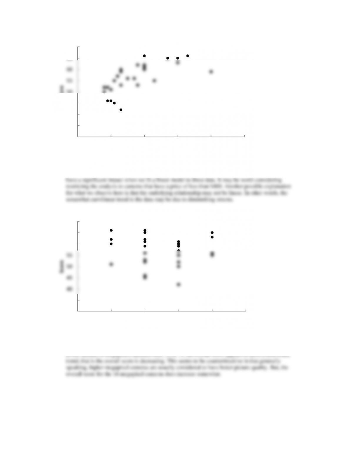
There appears to be a positive relationship between the price of the camera and the overall score.
But, observation 17, a Nikon camera with a price of $400, appears to be an observation that will
The number of megapixels does not appear to have much effect on the overall score. But, note that
as the number of megapixels increase from 10 to 14, the overall score appears to have a downward
30
35
40
45
50
55
60
65
70
0 100 200 300 400 500
Score
Price ($)
30
35
40
45
50
55
60
65
70
810 12 14 16 18
Score
Megapixels
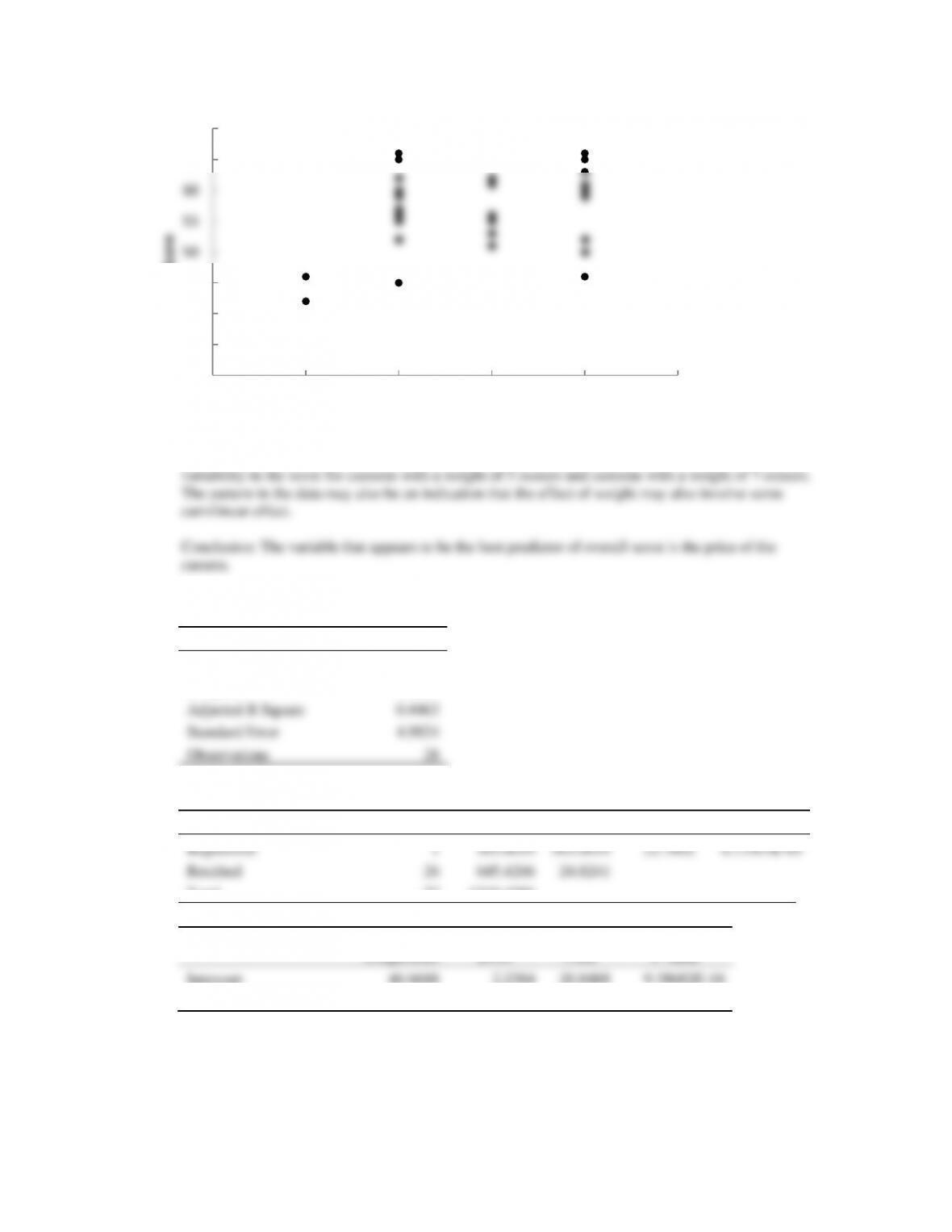
There may be a modest increase in overall score for cameras that weigh more. Also note the large
3. A portion of the Excel output follows:
Regression Statistics
Multiple R
0.6832
R Square
0.4668
Adjusted R Square
0.4463
Standard Error
4.9824
Observations
28
ANOVA
df
SS
MS
F
Significance F
Regression
1
565.0019
565.0019
22.7602
6.15507E-05
Residual
26
645.4266
24.8241
Total
27
1210.4286
Coefficients
Standard
Error
t Stat
P-value
Intercept
46.6688
2.2384
20.8488
9.38682E-18
Price ($)
0.0552
0.0116
4.7708
6.15507E-05
With a p-value = .000, price is a significant factor in predicting the overall score. The estimated
regression equation explained 46.68% of the variability in the overall score.
4. Using only the data for the Canon cameras, the scatter diagram using the price of the camera as the
independent variable follows.
30
35
40
45
50
55
60
65
70
345678
Score
Weight (oz.)
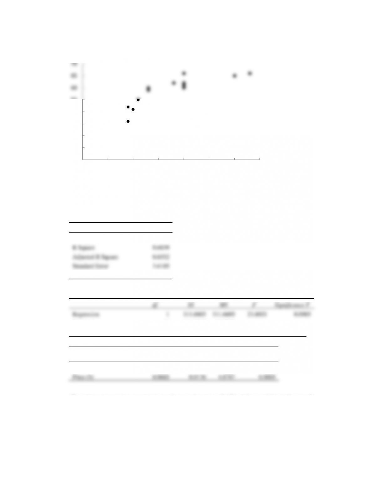
There does appear to be a relationship between the price of the camera and the overall score. But, the
relationship appears to be curvilinear. However, using simple linear regression for these data we
obtain the following output.
Regression Statistics
Multiple R
0.8270
R Square
0.6839
Adjusted R Square
0.6552
Standard Error
3.6185
Observations
13
ANOVA
df
SS
MS
F
Significance F
Regression
1
311.6605
311.6605
23.8021
0.0005
Residual
11
144.0319
13.0938
Total
12
455.6923
Coefficients
Standard
Error
t Stat
P-value
Intercept
47.2880
2.5729
18.3793
1.32053E-09
Price ($)
0.0665
0.0136
4.8787
0.0005
score using the price of the camera. But, the curvilinear relationship we observed in the scatter
diagram is still a concern. The issue whether the underlying relationship may be better described by
curvilinear model cannot be resolved using the methods introduced in this chapter.
30
35
40
45
50
55
60
65
70
050 100 150 200 250 300 350
Score
Price ($)
Case Problem 4: Finding the Best Car Value
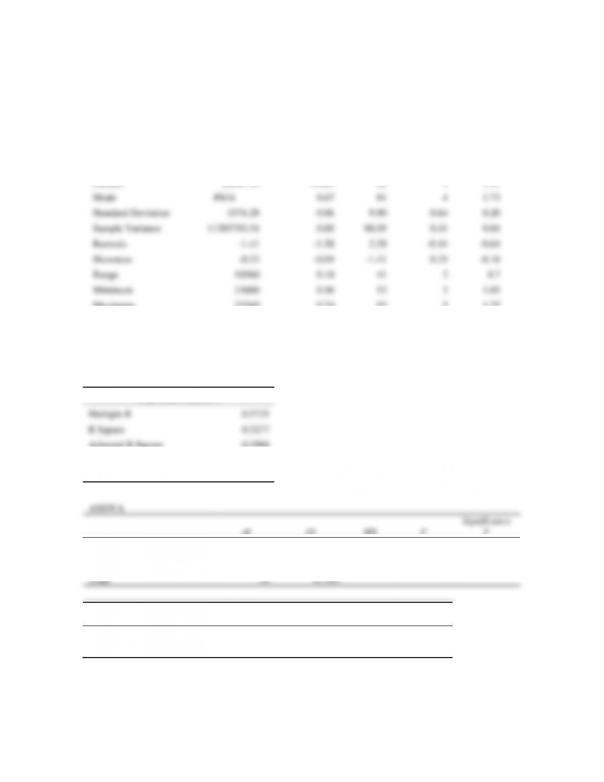
1. Descriptive statistics follow.
Price ($)
Cost/Mile
Road-
Test
Score
Predicted
Reliability
Value
Score
Mean
26886.20
0.642
80.45
3.75
1.46
Standard Error
754.51
0.01
2.21
0.14
0.04
Median
28067.50
0.665
82
4
1.43
Mode
#N/A
0.67
81
4
1.73
Standard Deviation
3374.28
0.06
9.90
0.64
0.20
Sample Variance
11385793.54
0.00
98.05
0.41
0.04
Kurtosis
-1.41
-1.58
2.58
-0.44
-0.64
Skewness
-0.23
-0.04
-1.41
0.25
-0.18
Range
10560
0.18
41
2
0.7
Minimum
21800
0.56
52
3
1.05
Maximum
32360
0.74
93
5
1.75
Sum
537724
12.84
1609
75
29.16
Count
20
20
20
20
20
2. A portion of the Excel output follows.
Regression Statistics
Multiple R
0.5725
R Square
0.3277
Adjusted R Square
0.2904
Standard Error
0.1663
Observations
20
ANOVA
df
SS
MS
F
Significance
F
Regression
1
0.2428
0.2428
8.7754
0.0083
Residual
18
0.4980
0.0277
Total
19
0.7407
Coefficient
s
Standard Error
t Stat
P-value
Intercept
2.3587
0.3063
7.7004
4.2026E-07
Price ($)
0.0000
0.0000
-2.9623
0.0083
3. A portion of the Excel output follows.
Regression Statistics
Multiple R
0.7164
R Square
0.5132
Adjusted R Square
0.4861
Standard Error
0.1415
Observations
20
ANOVA
df
SS
MS
F
Significance F
Regression
1
0.3801
0.3801
18.9741
0.0004
Residual
18
0.3606
0.0200
Total
19
0.7407
Coefficients
Standard
Error
t Stat
P-value
Intercept
2.9422
0.3422
8.5979
8.65063E-08
Cost/Mile
-2.3119
0.5307
–
4.3559
0.0004
4. A portion of the Excel output follows.
Regression Statistics
Multiple R
0.4116
R Square
0.1694
Adjusted R Square
0.1232
Standard Error
0.1849
Observations
20
ANOVA
df
SS
MS
F
Significance F
Regression
1
0.1255
0.1255
3.6704
0.0714
Residual
18
0.6153
0.0342
Total
19
0.7407
Coefficients
Standard Error
t Stat
P-value
Intercept
0.7978
0.3471
2.2986
0.0337
Road-Test Score
0.0082
0.0043
1.9158
0.0714
5. A portion of the Excel output follows.
Regression Statistics
Multiple R
0.3506
R Square
0.1229
Adjusted R Square
0.0742
Standard Error
0.1900
Observations
20
ANOVA
df
SS
MS
F
Significance F
Regression
1
0.0910
0.0910
2.5225
0.1296
Residual
18
0.6497
0.0361
Total
19
0.7407
Coefficients
Standard Error
t Stat
P-value
Intercept
1.0515
0.2594
4.0535
0.0007
Predicted Reliability
0.1084
0.0682
1.5882
0.1296
price ($) and value score (p-value = .0083). Reviewing the regression output in parts (3) – (5)
indicates that cost/mile is the best single predictor of value score (R-Sq = .5132). To further
investigate the relationship among these variables we really need to use multiple regression analysis.