6.* A restaurant wants to forecast its weekly sales. Historical data (in dollars) for fifteen weeks
are shown below and can be found on the worksheet C11P6 in the OM5 Data &
Calculations Workbook. (Note: you may copy the data from the worksheet to the appropriate
Excel template.)
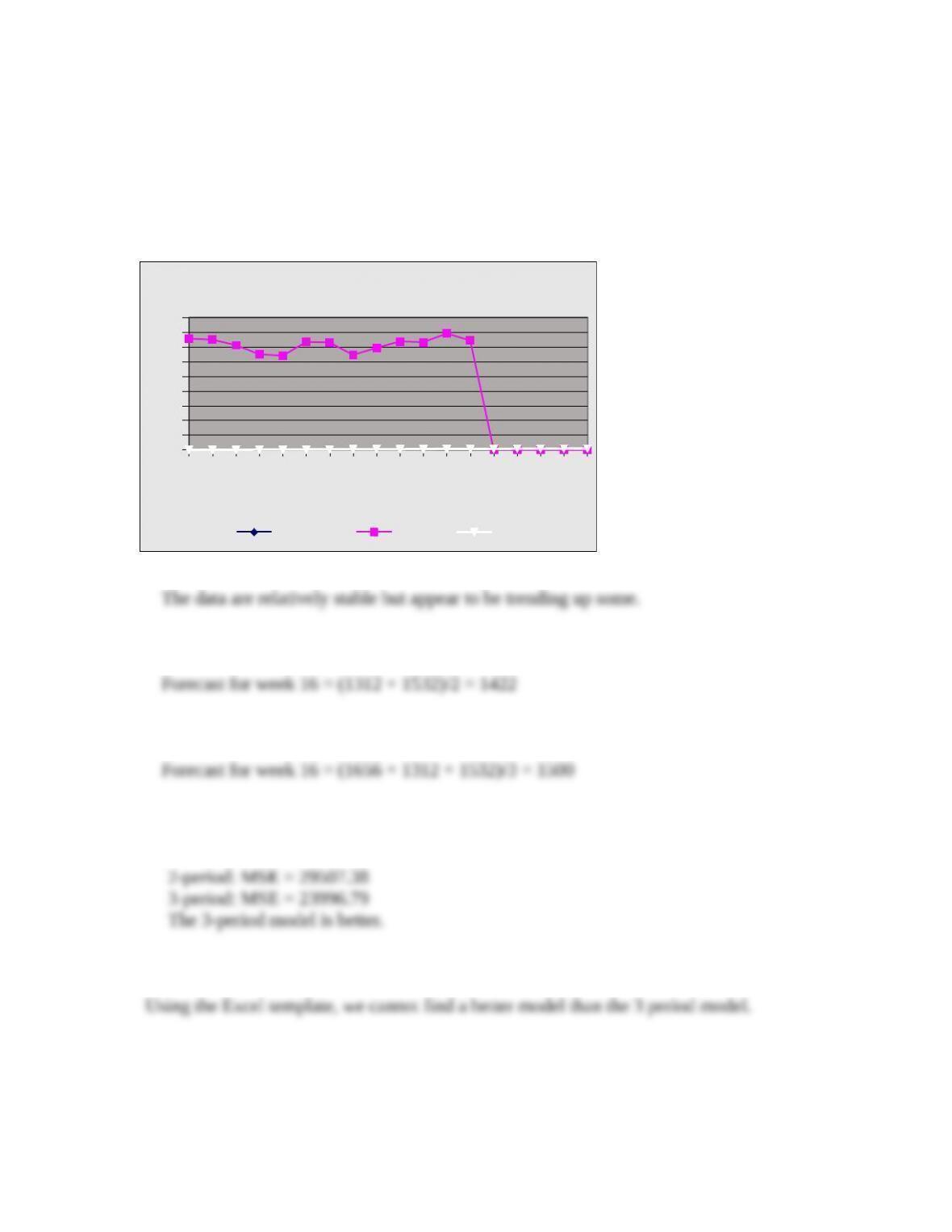
a. Plot the data and provide insights about the time series.
1 2 3 4 5 6 7 8 9 10 11 12 13 14 15
0
2 00
400
600
800
1000
12 00
1400
1600
1800
Moving Average Forecast
Observa tion Forecast
Time Pe rio d
b. What is the forecast for week 16, using a two-period moving average?
c. What is the forecast for week 16, using a three-period moving average?
d. Compute MSE for the two- and three-period moving average models and compare your
results.
e. Find the best number of periods for the moving average model based on MSE.
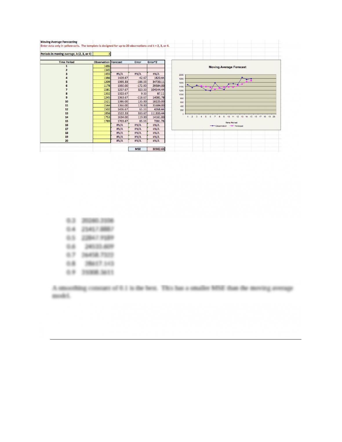
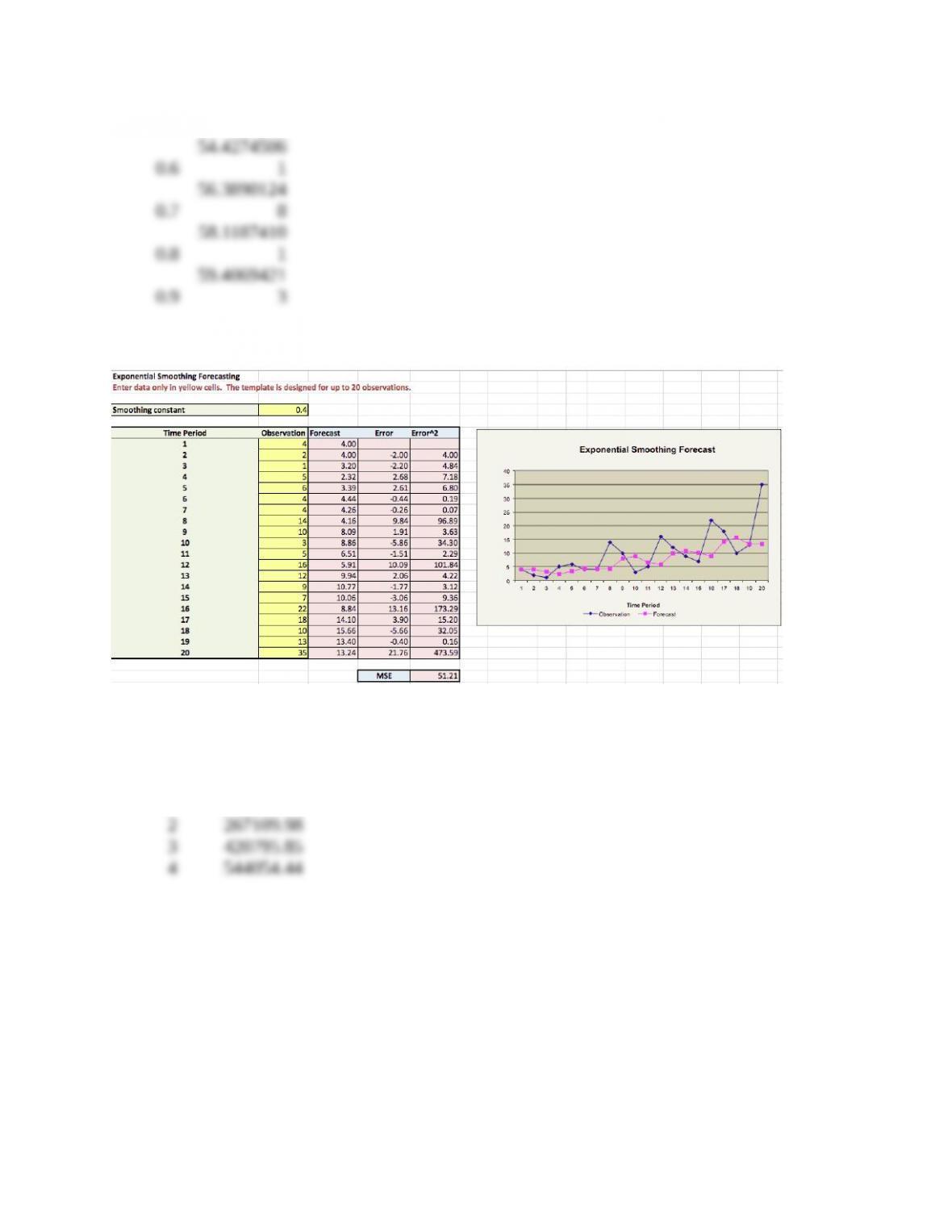
7.* For the data in Problem 6, find the best single exponential smoothing model by evaluating
the MSE for from 0.1 to 0.9, in increments of 0.1. How does this model compare with the
best moving average model found in Problem 6?
Alpha MSE
0.1 18670.5337
0.2 19358.3875
8.* The monthly sales of a new business software package at a local discount software store
were as follows:
Week 1 2 3 4 5 6 7 8 9 10
Sales 460 415 432 450 488 512 475 502 449 486
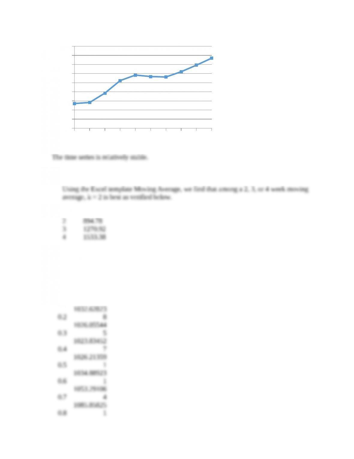
a. Plot the data and provide insights about the time series.
1 2 3 4 5 6 7 8 9 10
14000
14500
15000
15500
16000
16500
17000
17500
18000
18500
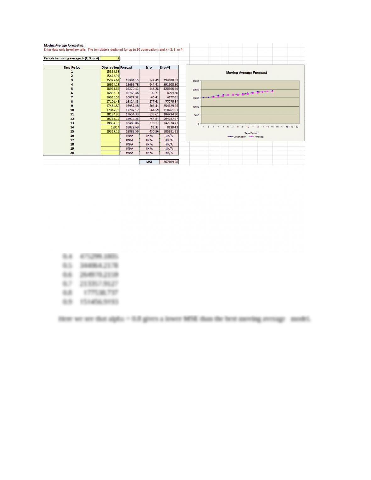
b. Find the best number of weeks to use in a moving-average forecast based on MSE.
k MSE
c. Find the best single exponential smoothing model to forecast these data.
Using the Excel template Exponential Smoothing, we find:
Alpha MSE
0.1
1039.08017
7
9.* Consider the quarterly sales data for Worthington Health Club shown here (also available on
the worksheet C11P9 in the OM4 Data Workbook):
Quarter Total
Year 1 2 3 4 Sales
1 4 2 1 5 12
2 6 4 4 14 28
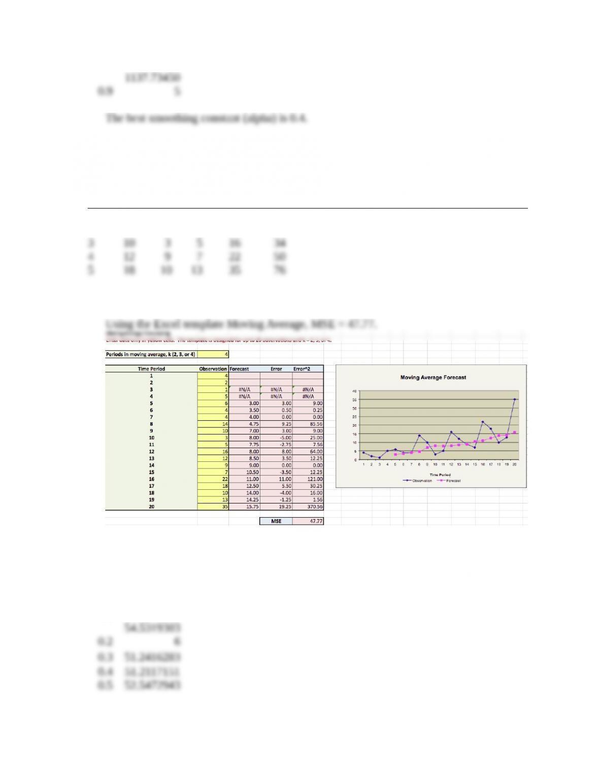
a. Develop a four-period moving average model and compute MSE for your forecasts.
b. Find a good value of for a single exponential smoothing model and compare your
results to part (a).
Alpha MSE
0.1
66.5359439
4
2
The moving average forecast provides a smaller MSE.
10.* Using the factory energy cost data in Exhibit 11.11, find the best moving average and
exponential smoothing models. Compare their forecasting ability with the regression
model developed in the chapter. Which model would you choose and why?
k MSE
For the moving average models, k = 2 is best.
For exponential smoothing:
Alpha MSE
0.1 2437086.953
0.2 1218910.64
0.3 716342.3987
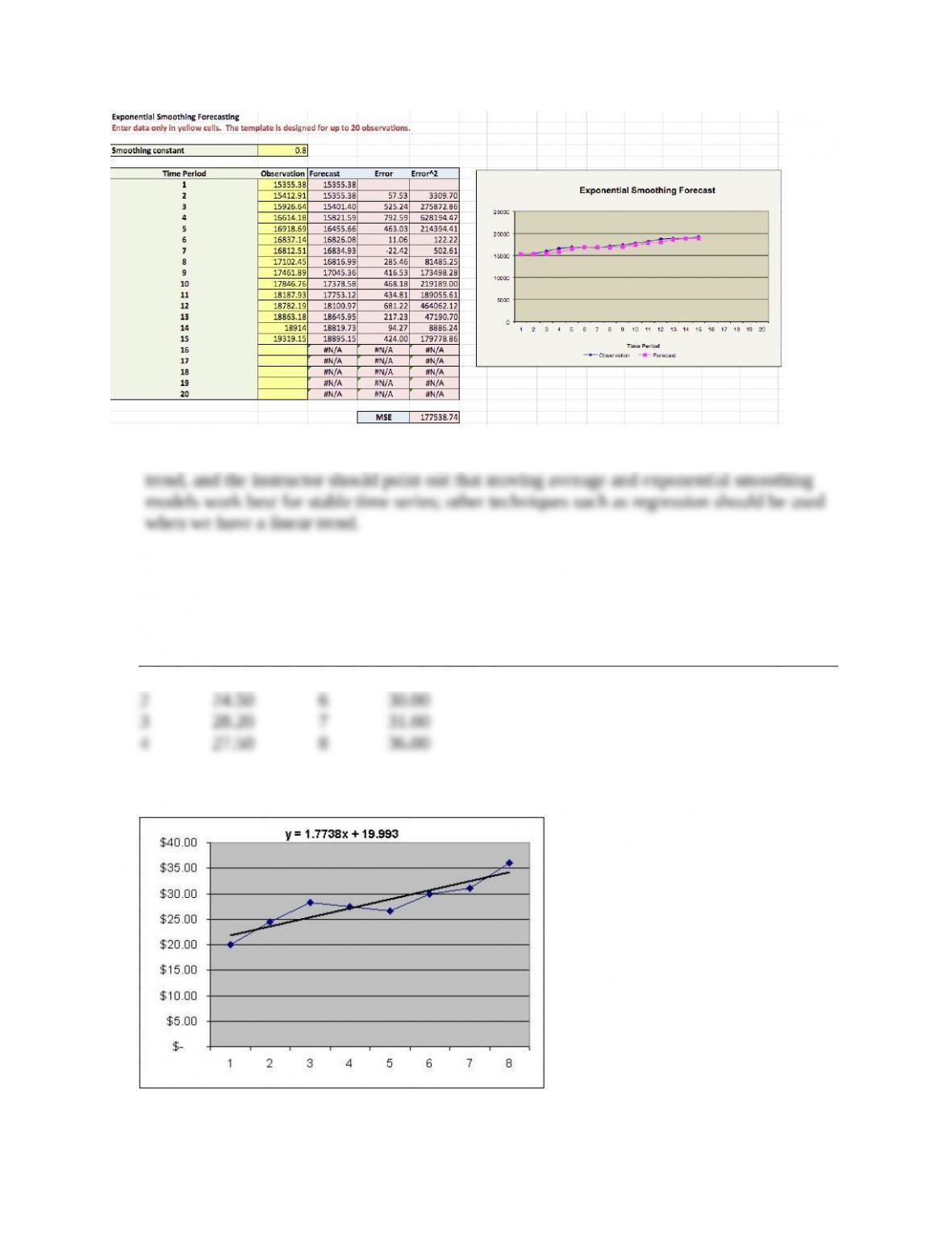
Note that in both cases, the forecasts lag the data. This occurs because we have a linear
11. The president of a small manufacturing firm is concerned about the continual growth in
manufacturing costs in the past several years. The data series of the cost per unit for the
firm’s leading product over the past eight years are given as follows:
Year Cost/Unit ($) Year Cost/Unit ($)
1 20.00 5 26.60
a. Construct a chart for this time series. Does a linear trend appear to exist?
Yes, a linear trend is apparent.
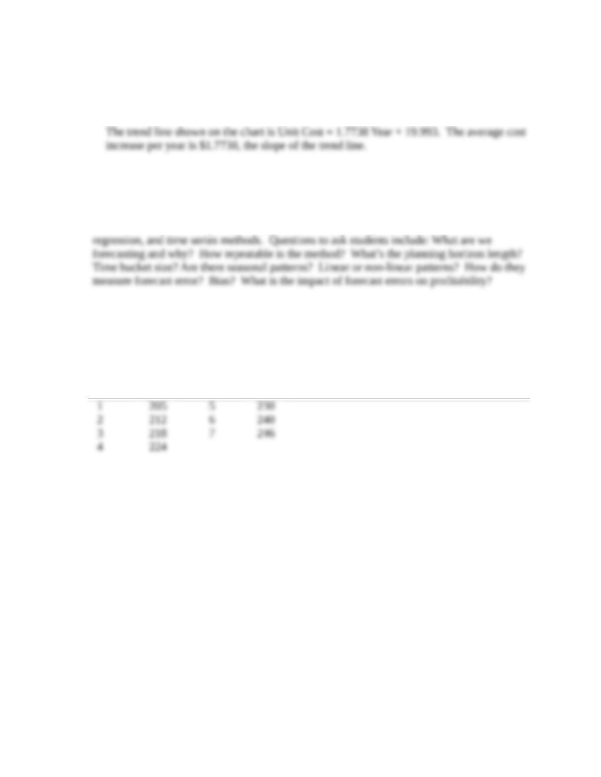
b. Develop a simple linear regression model for these data. What average cost increase has
the firm been realizing per year?
12. Interview a current or previous employer about how he or she makes forecasts. Document in
one page what you discovered, and describe it using the ideas discussed in this chapter.
Students will find companies and managers who use a wide range of methods to make
forecasts such as the Delphi Method, grass roots forecasting, linear and non-linear
13. Canton Supplies, Inc., is a service firm that employs approximately 100 people. Because of the
necessity of meeting monthly cash obligations, the Chief Financial Officer wants to develop a
forecast of monthly cash requirements. Because of a recent change in equipment and operating
policy, only the past seven months of data are considered relevant.
Cash Required Cash Required
Month ($1,000) Month ($1,000)
7654321
250
240
230
220
210
200
Month
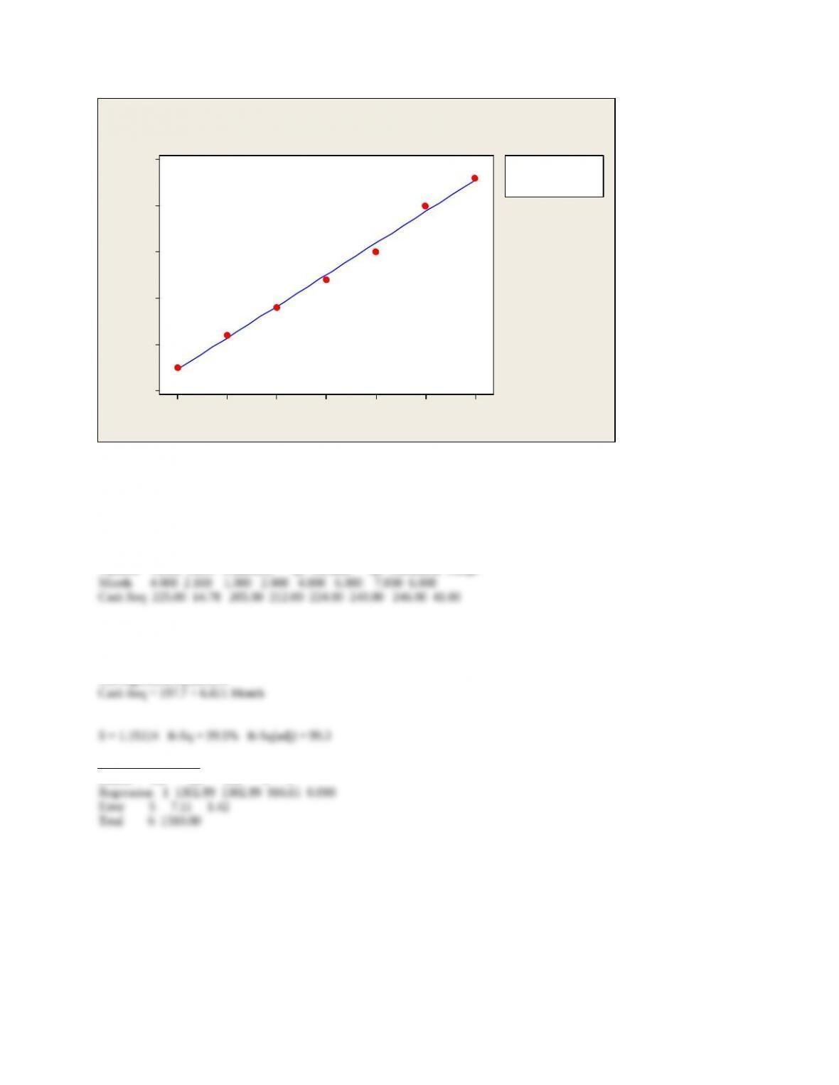
Cash Req
S 1.19224
R-Sq 99.5%
R-Sq(adj) 99.3%
Fitted Line Plot
Cash Req = 197.7 + 6.821 Month
Too perfect to be true! Simple regression. The CFO can make almost a perfect forecast of
monthly cash flow.
Descriptive Statistics: Month, Cash Req
Variable Mean StDev Minimum Q1 Median Q3 Maximum Range
Regression Analysis: Cash Req versus Month
The regression equation is
Analysis of Variance
Source DF SS MS F P
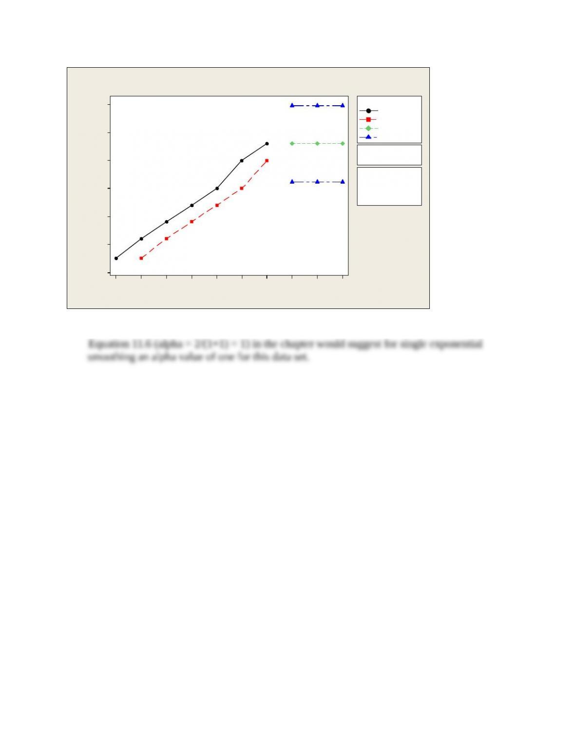
Moving Average for Cash Req
10987654321
260
250
240
230
220
210
200
Index
Cash Req
Length 1
Moving Average
MAPE 2.9912
MAD 6.8333
MSD 48.8333
Accuracy Measures
Actual
Fits
Forecasts
95.0% PI
Variable
Moving Average Plot for Cash Req