
Chapter 11 Principles of Finance 6e
Besley/Brigham
11–12
The T-bills are risk-free in the default risk sense because the 8 percent return will be
realized in all possible economic states. However, remember that this return is composed
(2) High Tech’s returns move with, and thus are positively correlated with, the economy,
b. The expected rate of return,
r
ˆ
, is expressed as follows:
=
=
n
1i
ii rr
ˆPr
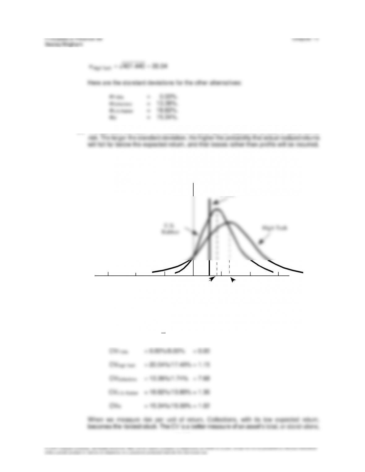
c. (1) The standard deviation is calculated as follows:
i
n
1i
2
i
2)r
ˆ
r( Pr
=
−==
440.401276.106952.61704.2272.75236.155
%)4.17%0.50(1.0%)4.17%0.35(2.0
%)4.17%0.20(4.0%)4.17%0.2(2.0%)4.17%0.22(1.0
22
2222
Tech High
=++++=
−+−+
−+−−+−−=
11–13
(2) The standard deviation is a measure of a security’s (or a portfolio’s) total, or stand-alone,
(3) Probability distribution curves for High Tech, U.S. Rubber, and T-bills are shown here:
–45 –30 –15 15 30 45
13.8 17.4
T-bills
High Tech
U.S.
Rubber
Probability
Rate of
Return
(%)
d. The coefficient of variation (CV) is a standardized measure of dispersion about the expected
value; it shows the amount of risk per unit of return.
r
ˆ
CV
Variation
of tCoefficien
==

Chapter 11 Principles of Finance 6e
11–14
e. (1) To find the expected rate of return on the two-stock portfolio, we first calculate the rate of
return on the portfolio in each state of the economy. Because we have half of our money in
the other states of the economy, and get these results:
State Portfolio
Recession 3.00%
Alternatively, we could apply this formula:
The standard deviation of the portfolio is:
129.11948.2717.1074.0074.2316.4
%)57.9%0.15(1.0%)57.9%50.12(2.0
%)57.9%00.10(4.0%)57.9%35.6(2.0%)57.9%00.3(1.0
22
2222
P
=++++=
−+−+
−+−+−=
%336.3129.11
P==
CVP = 3.336%/9.57% = 0.349
(2) Using either σ or CV as our total risk measure, the total risk of the portfolio is significantly
Principles of Finance 6e Chapter 11
Besley/Brigham
11–15
f.
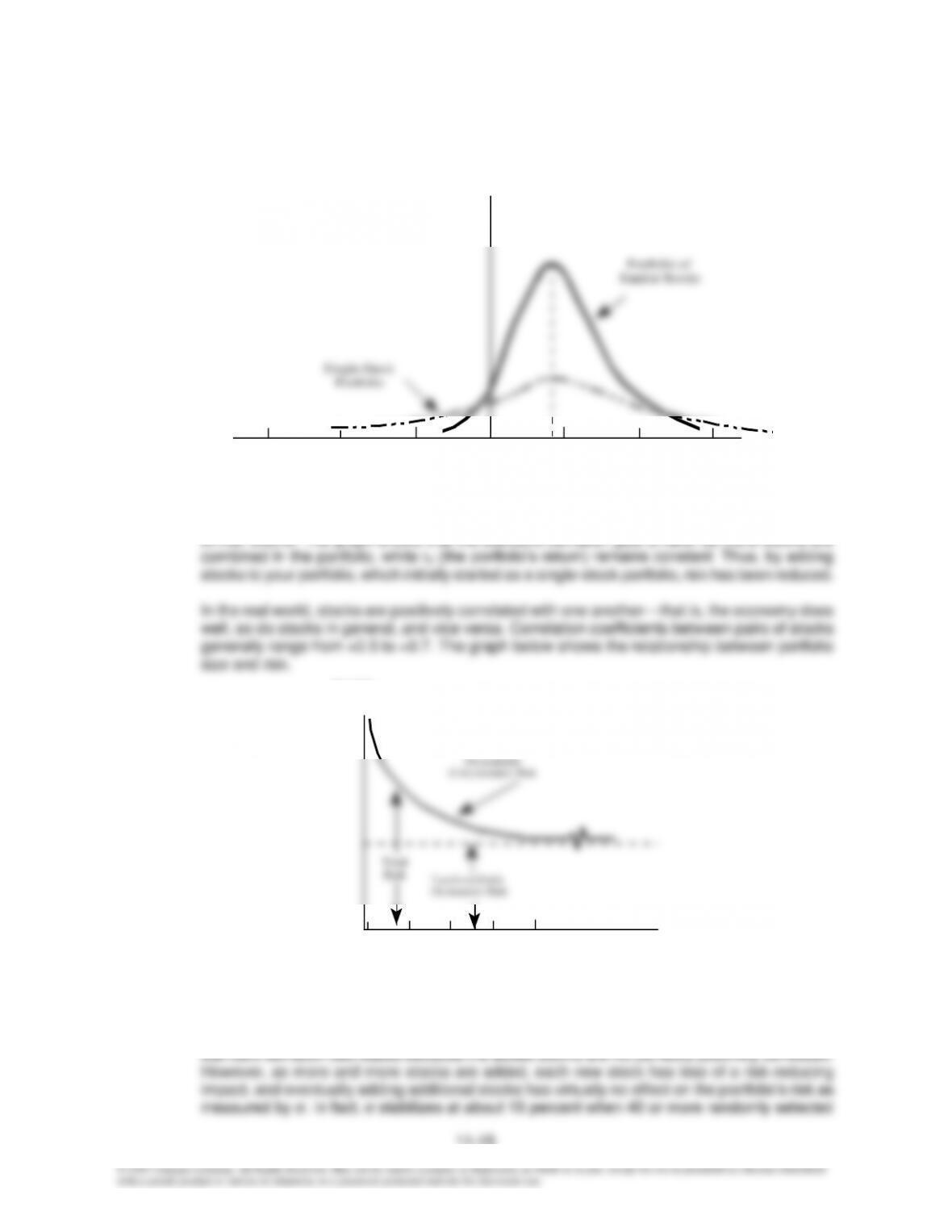
–45 –30 –15 15 30 45
Probability
Rate of
Return
(%)
Portfolio of
Similar Stocks
Single-Stock
Portfolio
This graph shows the probability distributions for a one-stock portfolio and a portfolio of many
similar stocks. The graph shows that the standard deviation gets smaller as more stocks are
Portfolio
Risk, FP (%)
Number of
Stocks
Total
Risk Nondiversifiable
(Systematic) Risk
Diversifiable
(Unsystematic) Risk
10 20130 40

Chapter 11 Principles of Finance 6e
Besley/Brigham
11–16
g. (1) Portfolio diversification does affect investors’ views of risk. A stock’s total, or stand-alone,
risk as measured by its σ or CV, might be important to an undiversified investor, but it is not
(2) If you hold a one-stock portfolio, you will be exposed to a high degree of risk, but you won’t
h. (1) Draw the framework of the graph, put up the data, plot the points for the market (45° line)
and connect them, and then get the slope as δY/δX = 1.0.) State that an average stock, by
(3) We do not yet have enough information to choose among the various alternatives. We
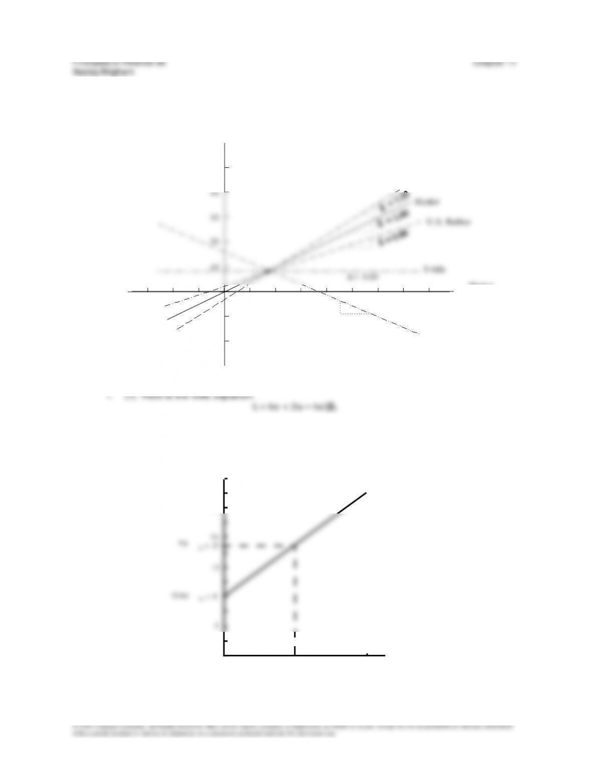
(4)
-10 10 20 30 40
50
40
30
20
10
-10
-20
Stock
Return
(%)
Market
Return
(%)
High Tech
Market
U.S . Rubber
T-bills
Collections
ß = -0.86
ß = 0.00
•
Characteristic Lines
If we use the T-bill yield as a proxy the risk-free rate, then rRF = 8%. Further, our estimate
of rM =
r
ˆ
is 15%. Thus, the SML is drawn as follows:
24
20
16
12
k
(%)
kM = 15
SML
r
(%)
rM
Chapter 11 Principles of Finance 6e
Besley/Brigham
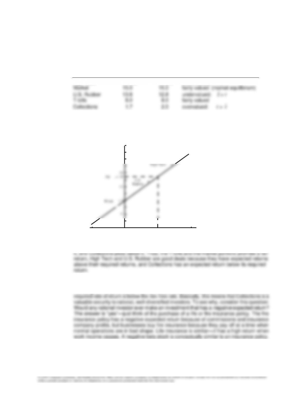
(2) Using the SML equation, we have the following relationships:
Expected Required
Return Return
Security (
r
ˆ
) (r) Condition
High Tech 17.4% 17.0% undervalued:
r
ˆ
> r
r
ˆ
These returns are plotted on the SML graph next.
012
24
20
16
12
kT-BILLS = 8
4
B eta ( ß )
k
(%)
kM = 15
SML
•
•
Hig h Tec h
U.S.
R ub ber
-1
•C ol lec ti on s
•
•
The T-bills and market portfolio plot on the SML, High Tech and U.S. Rubber plot above
(3) Collections is an interesting stock. Its negative beta indicates negative market risk—
including it in a portfolio of “normal” stocks will lower the portfolio’s risk. Therefore, its
r
(%)
rM
rT-bill

Principles of Finance 6e Chapter 11
Besley/Brigham
j. (1) This effect is graphed next.
012
24
20
16
12
8
4
B ETA ( ß )
k
(%)
C HA N GES I N TH E S ML
-1
ORIGINAL
SITUATION
IN CR EASED
INFLATION
IN CR EASED
R ISK AVER SION
Here we have plotted the SML for betas ranging from 0 to 2.0. The base case SML is
r (%)

Chapter 11 Principles of Finance 6e
Besley/Brigham
Stock A Stock B Stock C Portfolio
2011 –18.00% –14.50% 32.00% –0.17%

Principles of Finance 6e Chapter 11
Besley/Brigham
11–21
• Should RIP be more concerned with return than risk when making its decision about the PAIDs?
This question follows the above discussion. The short, simple answer is “absolutely not.” There are
• If the PAIDs are recommended, what should RIP tell its customers?
RIP could find itself in a great deal of trouble, both financially and legally, if it doesn’t fully disclose any
• Would you recommend the PAIDs?
References:
The scenario presented here parallels the well-publicized cases of (1) Orange County, California that came
to light in 1994 and (2) Long-Term Capital Management L.P. Orange County lost billions of dollars with its
investment fund, apparently because the managers of the fund did not fully understand the risk ramifications
of some of the investments in the portfolio, especially derivatives. Long-Term Capiôal Management L.P.,
which employed complex arbitrage strategies to construct investment qosi|ions that were suppose to
generate positive returns in any type of market, was “bailed out” of bankruptcy only after large financial
institutions provided nearly $4 billion.
The following articles offer interesting insights into what caused Orange County’s problems:
“Untangling the Derivative Mess,” Fortune, March 20, 1995, p. 50+.
“Orange County is Looking Green Around the Gills,” Business Week, December 26, 1994, p. 66+.
“Derivatives Lead to a Huge Loss in Public Fund,” The Wall Street Journal, December 2, 1994, p. A3+.
“Bitter Fruit in Orange County,” Business Week, May 30, 1994, p. 44+.
The following articles describe some of the complexities and the reasons for the trouble at Long-Term
Capital Management L.P.:
“Failed Wizards of Wall Street: Can You Devise Surefire Ways to Beat the Markets? The Rocket Scientists
Thought They Could. Boy Were They Wrong,” Business Week, September 21, 1998, p. 114.
“Bailout Blues: How a Big Hedge Funds Marketed Its Expertise and Shrouded Its Risk; Regulators and

Chapter 11 Principles of Finance 6e
Besley/Brigham
Lenders Knew Little About the Gambles At Long-Term Capital; ‘Stardust in Investors’ Eyes,” The Wall Street
Journal, September 25, 1998, p. A1+.
“A House Built on Sand. John Meriwether’s Once-Mighty Long-Term Capital Has All But Crumbled. So Why
Did Warren Buffett Offer to Buy It?,” Fortune, October 26, 1998, p. 110+.