ADDITIONAL ISSUES FOR CLASSROOM DISCUSSION
1. Students may find the AD-AS model dicult at first. However, once
2. You can expand on the discussion of policy in this chapter. Monetary
and fiscal policy work in similar ways, though (at least in the short
run) they have di’ering implications for the real interest rate.
Because this chapter does not develop the IS and LM models, as is
done in a course in intermediate macroeconomics, the mechanism
for analyzing the impact on the real interest rate is not readily
apparent. But you could discuss it intuitively, noting that
expansionary monetary policy reduces the real interest rate (as
discussed in Chapter 11), while expansionary fiscal policy might
increase the real interest rate.
3. The discussion of rational expectations in this chapter is fairly short
and terse. However, you could easily expand on it to discuss how
the modeling of expectations had been considered fairly
unimportant in the large, structural macroeconomic models. But
once economists discovered the importance of expectations, many
of them devoted their research e’orts to it and developed many
useful models. You could discuss how cross-equation restrictions
were developed from such models and the need for econometric
methods that could be used to estimate complete models with
rational expectations.
SOLUTIONS TO TEXTBOOK ANALYTICAL PROBLEMS
11. A decrease in government defense spending represents a reduction
Chapter 12: The Aggregate-Demand/Aggregate-Supply Model 127
14. The increase in the wealth of consumers increased current and
Chapter 12: The Aggregate-Demand/Aggregate-Supply Model 128
ADDITIONAL TEACHING NOTES
Using the AD-AS Model Numerically
In the last part of this chapter, we’ll examine large, structural
macroeconomic models of the economy. To give you a feel for what
those models are like, in this section we’ll add some actual numbers to
go along with the curves. The results of the model can then be
expressed either analytically (using graphs as we’ve already been
doing) or numerically (using equations and numbers).
Chapter 12: The Aggregate-Demand/Aggregate-Supply Model 129
Here is an example of a numerical AD-AS model. Some of the elements
discussed earlier are assumed away, so we won’t need to deal with as
many elements. The numbers are made up to make the numbers come
out reasonably; they don’t necessarily represent the actual economy.
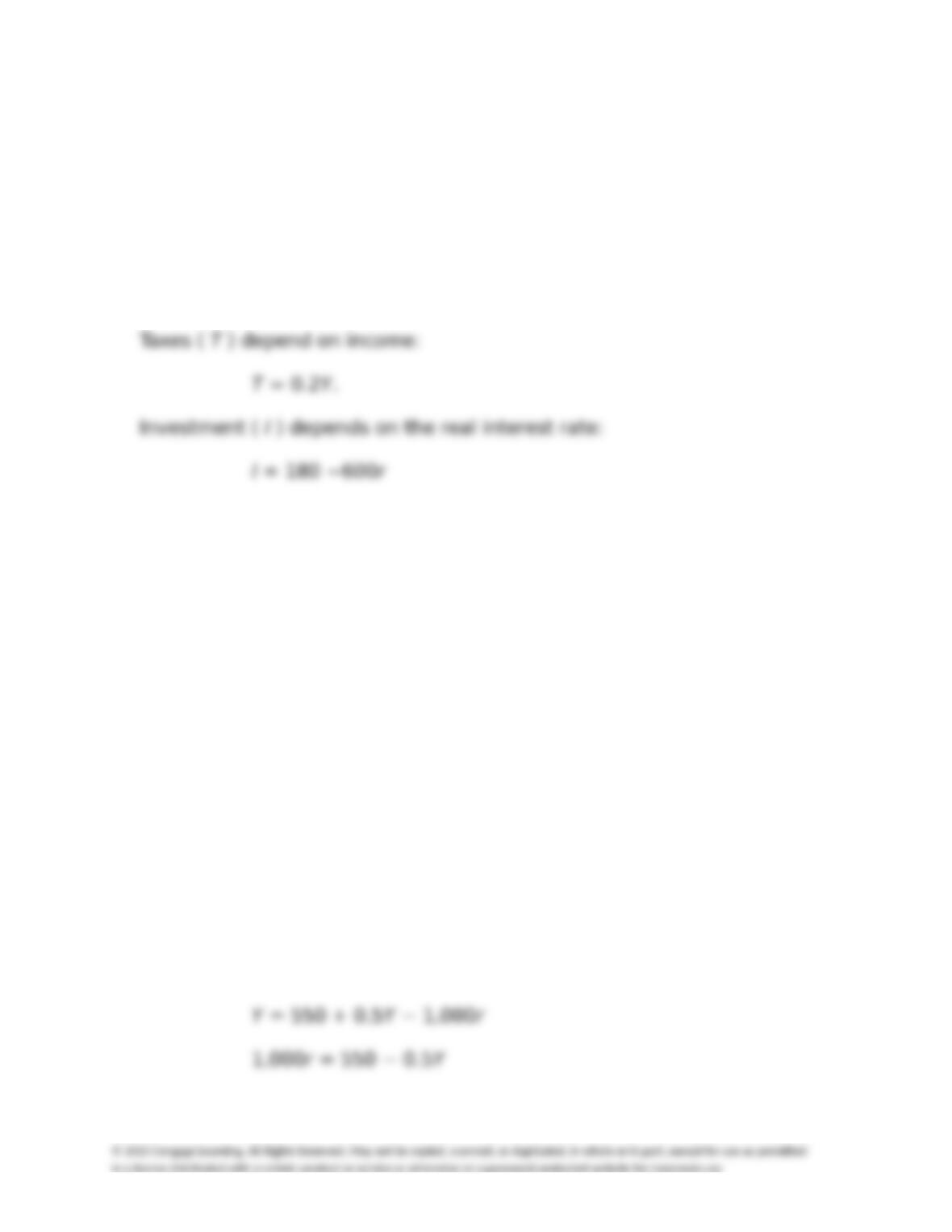
Consumption spending (C) depends on current after–tax income (Y −T)
and the real interest rate ( r ):
C = 100 +0.75(Y − T) − 400r
Net exports depend on income in the U.S. and in foreign countries:
NX = −0.1Y + 0.1YF
YF = 700
Government spending is set by the government at a particular level
that doesn’t depend on anything else:
G = 200
Using the fact that Y = C + I + G + NX and substituting in for C, I, G,
and NX, we get
Y = C + I + G + NX
= {100 + [0.75(Y − 0.2Y)] − 400r}+ {180 − 600r}+ {200}+
{−0.1Y + (0.1 × 700)}
= 550 + 0.5Y − 1,000r
Solving this equation for r in terms of Y gives
Chapter 12: The Aggregate-Demand/Aggregate-Supply Model 130
r = 0.55 − 0.0005Y
(1)
Equation (1) shows the relationship between the real interest rate and
income that clears the market for goods and services.
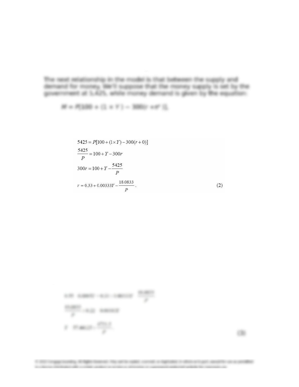
where πe is the expected in<ation rate. Equating the money supply to
money demand and assuming that expected in<ation equals 0 give a
relationship between income, the real interest rate, and the price level:
Equation (2) shows the relationship between the real interest rate,
income, and the price level, which is consistent with equilibrium in the
money market. For a given price level, equation (2) is a second
relationship [the first being equation (1)] between the real interest rate
and income.
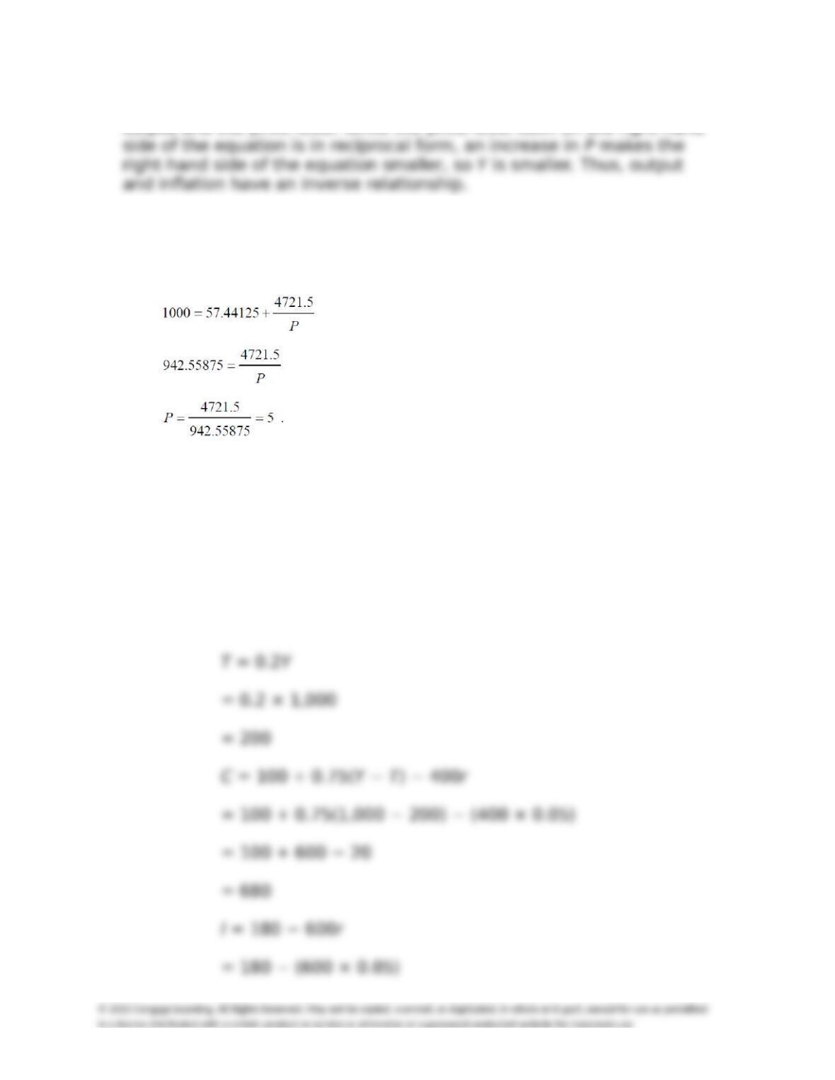
Next, we need to combine the information in equations (1) and (2) to
get the aggregate demand curve. Since both equations (1) and (2) are
in terms of the real interest rate on the left-hand side of the equations,
we can equate the right-hand sides of the two equations, yielding a
relationship between the price level and income (which is equal to
output):
Chapter 12: The Aggregate-Demand/Aggregate-Supply Model 131
Equation (3) represents the AD curve, which is a relationship between
output and the price level. Since the price-level term on the right-hand
In the long run, output equals potential output ( Ȳ ), which we’ll
suppose equals 1,000.
Plugging 1,000 into equation (3), we get
We can then use these results of Y = 1,000 and P = 5 to find out what
happens to the other variables. From equation (1), the real interest rate
( r ) is
r = 0.55 − (0.0005 × 1,000) = 0.05 ,
so r = 5 percent.
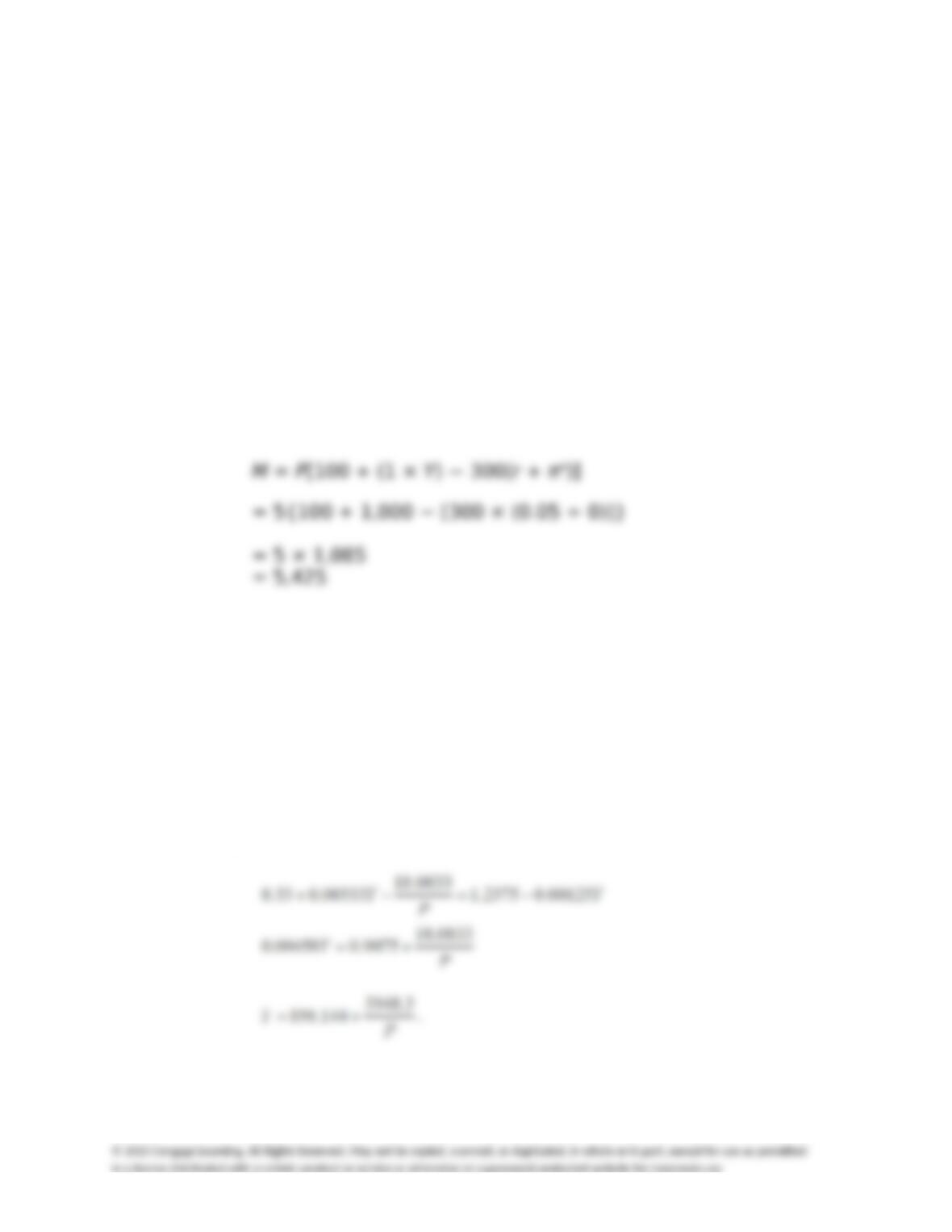
The other variables are:
Chapter 12: The Aggregate-Demand/Aggregate-Supply Model 132
= 150
NX = −0.1Y + 0.1YF
= (−0.1 × 1000) + (0.1 × 700)
= −30
Note that the components of output add up to the amount of output:
C + I + G + NX = 680 + 150 + 200 − 30
= 1,000
Note also that money demand equals money supply (M = 5,425):
In this model, as we saw with our figures, the variables can all change
when there is some change in one of the equations. To give an
example of this, let’s suppose that investment spending declines
substantially because business firms become pessimistic about their
future prospects. Investment falls to I = 125. In the short run, with the
expected price level still at 5, the decline in business optimism
changes equation (1):
r = 1.2375 − 0.00125Y.
Combining this equation with equation (2), we have the new AD curve:
The SRAS curve relates output in the short run to the price level:
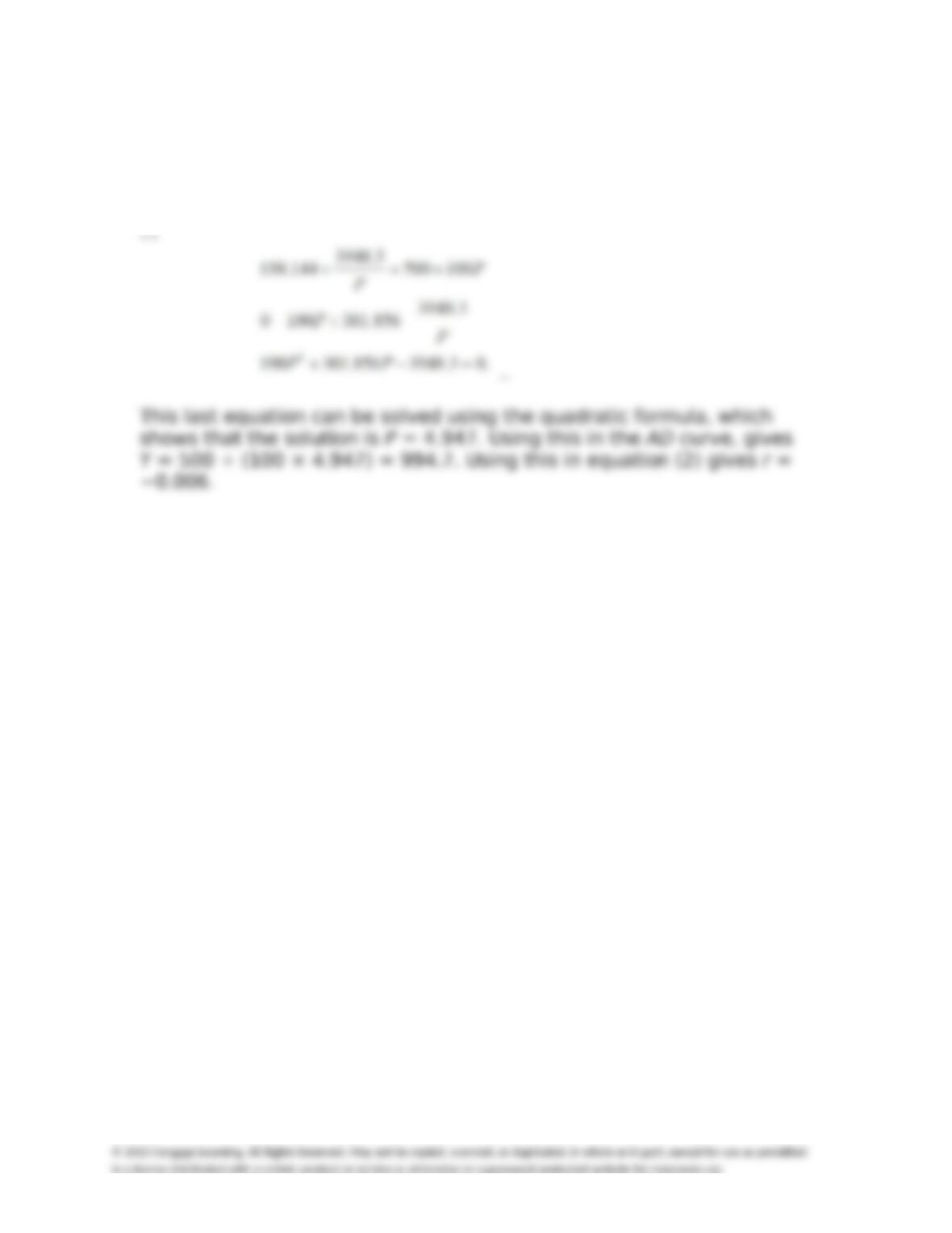
Chapter 12: The Aggregate-Demand/Aggregate-Supply Model 133
Y = 1,000 + 100(P − 5)
= 500 + 100P
Combining the AD curve and the SRAS curve gives: