ADDITIONAL ISSUES FOR CLASSROOM DISCUSSION
1. Take a poll of your students’ expectations for major macroeconomic
variables and the probability of a decline in real GDP for the next quarter.
2. Over the last 10 years, the labor force participation rate has trended
down signi.cantly, as Figure 10.3 shows. Discuss the difficulty of
determining trends at the end of a sample of data, when no one knows
what will happen to the variable next. For example, note the slight
downward trend in the early 1960s, which was only temporary.
3. Discuss why we need a committee to determine when business cycles
begin and end. Even looking at just the data in this chapter, not all
variables change direction at the o0cial peaks and troughs of the cycle.
You can look at the NBER’s web site (www.nber.org) to see some of the
current discussion about the state of the business cycle by the business
cycle dating committee.
ANSWERS TO TEXTBOOK NUMERICAL
EXERCISES AND ANALYTICAL PROBLEMS
Numerical Exercises
11. a. Working-age population ÷ population = 83/127 = 0.654 = 65.4
Chapter 10: Economic Growth and Business Cycles 106
Chapter 10: Economic Growth and Business Cycles 107
15. If you retire at age seventy, you will have worked for forty-nine years. If
Analytical Problems
16. Per-capita growth (growth rate of output per person) matters for
well-being; per-capita growth rate = output growth rate − growth rate of
population.
Country A: per-capita growth rate = 6% − 4% = 2%
Country B: per-capita growth rate = 4% − 1% = 3%
Thus, people in country B are better oH because their output per person
is rising faster.
Chapter 10: Economic Growth and Business Cycles 108
d. The labor force as a fraction of the population increases because
people re-enter the labor force when wages increase and jobs are
plentiful.
All four of these factors cause output to grow more rapidly in expansions.
ADDITIONAL TEACHING NOTES
What Causes Productivity to Change?
Chapter 10: Economic Growth and Business Cycles 109
A Simple Model of Economic Growth
Economists have studied economic growth and its causes for many years. In
1958, Nobel laureate
Robert Solow proposed a simple way to identify some of the factors that
cause the economy to grow. His model has been modi.ed and updated over
the past forty-.ve years, but the basic idea of the model remains clear and
convincing. Output depends on the amount of capital and labor, and
businesses can only buy new capital if they can borrow from people who
save.
Output in the Solow model is produced with capital and labor according to
the production function that we used earlier in equation
Yt = F(Kt, Lt), (7)
where we have added the subscripts t to indicate that the equation shows
the relationship between capital, labor, and output at a date t . The model is
one that accounts for the movements of output, capital, and labor over
time, so the subscript is needed to keep track of the values of the variables
at diHerent dates.
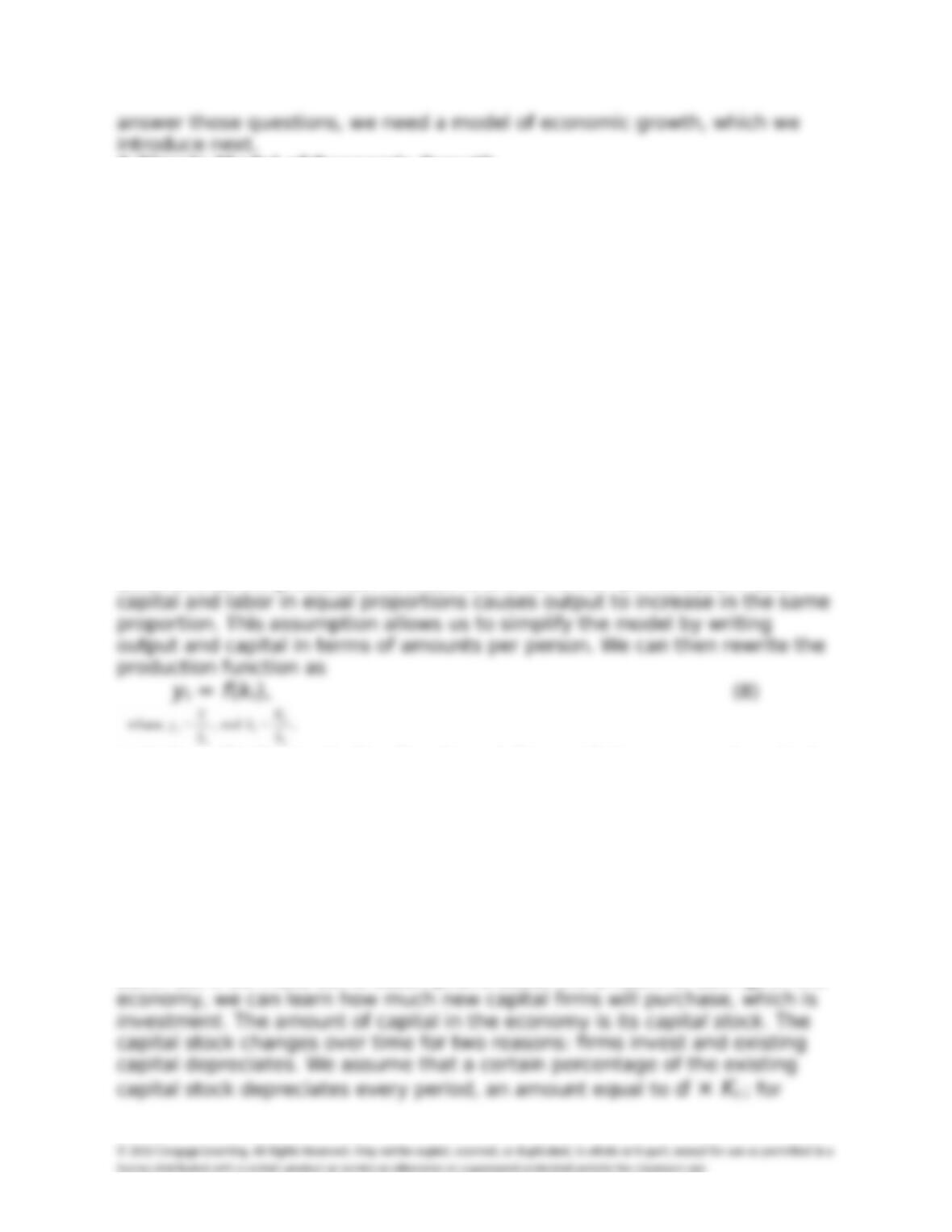
We make some assumptions that make the model easy to understand. We
assume that the production function is one for which an increase in both
and where f is the production function relating capital per person to output
per person. We assume that this production function has some standard
properties, namely that as the ratio of capital to labor (k) increases, the
ratio of output to labor (y) also increases, but by decreasing amounts.
Our next task is to .gure out what determines the amount of capital per
person. To do this, we use the assumption that businesses can only buy new
capital if someone saves. For example, a small business .rm’s owners might
save and buy new capital, a corporation could retain some of its earnings,
or a .rm could borrow funds from a bank, which is transferring those funds
from a number of individual savers who have deposited their savings in the
bank. So, if we make some assumptions about the amount of savings in the
Chapter 10: Economic Growth and Business Cycles 110
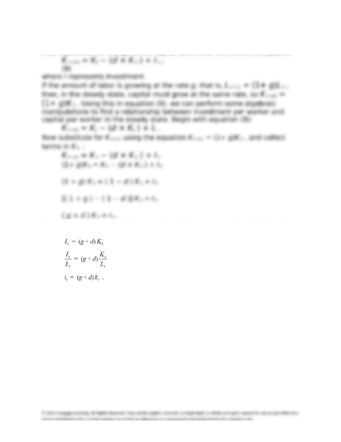
example, if capital depreciates 15 percent every year, then d = 0.15. We
thus represent the change of the capital stock over time with the equation
Now, if we switch around the two sides of the equation, then divide both
sides by L t , and use the de.nitions that y = Y/L and i = I/L, then we have
(10)
We make one more assumption, which is that in the long run the economy
will reach a steady state, a situation where capital, labor, and output are
growing at the same rate. This means that many of the variables that we
have de.ned, namely those in lowercase letters that represent output per
worker, capital per worker, and investment per worker, will not change over
time, so we can drop the time subscripts in equations (8) and (10). The
main equations of the model are now
y = f(k) (11)
and
i = (g + d )k . (12)
The last equation means that to keep the capital stock growing at the rate
that would maintain a constant ratio of capital to labor, investment per
worker (i) must equal the growth rate of the population plus the
depreciation rate on capital times the amount of capital per worker. The .rst
amount (the population growth rate) reUects the investment needed to
Chapter 10: Economic Growth and Business Cycles 111
make the capital stock increase at the same rate as population growth. The
second amount (the depreciation rate) represents the amount of investment
needed to replace machinery and equipment that has worn out.
For investment to occur, however, people must save. We will make the
same assumption that Solow did, namely, that savings per person (s) is a
constant fraction (v) of output per person. That is,
s = v × y. (13)
In this equation, v is the fraction of income that people save, and we
assume it is constant over time.
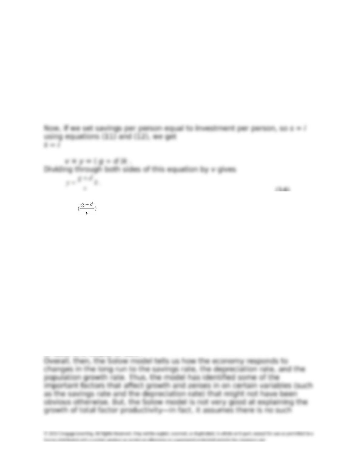
(14)
So, for savings to equal investment, output per person must equal a
constant times the amount of capital per person. Equations (11) and
(14) now give us two equations relating y and k, which we can use to solve
for their values.
In this model, the equilibrium values of y and k depend on the growth rate
of labor ( g ), the depreciation rate ( d ), and the savings rate ( v ). A higher
value of g or d, or a lower value of v , would mean that the right-hand side
of equation (14) would be higher for any given value of k .
There is some good intuition for these results. Consider two economies that
are identical in every way, except that one has greater population growth
than the other. With greater population growth, it takes more savings to
maintain a given ratio of capital to labor. Because savings is a .xed
proportion of output, an economy with greater population growth would
have a lower ratio of capital to labor, and hence a lower ratio of output to
labor. Similarly, an economy in which capital depreciates faster will also
have lower k and y in equilibrium.
On the other hand, an economy that has a higher savings rate out of
income will invest more, and in equilibrium will have a higher ratio of capital
to labor and output to labor.
Chapter 10: Economic Growth and Business Cycles 112
growth. The model only explains the growth in labor productivity that arises
because of additional capital relative to labor.
Models with Total Factor Productivity Growth
A major shortcoming of the Solow model is that although the economy
grows, it does so (in the long run) at the rate of population growth, because
in the steady state the ratio of output to labor is constant. Are economies
doomed to grow no faster or slower than their populations grow?
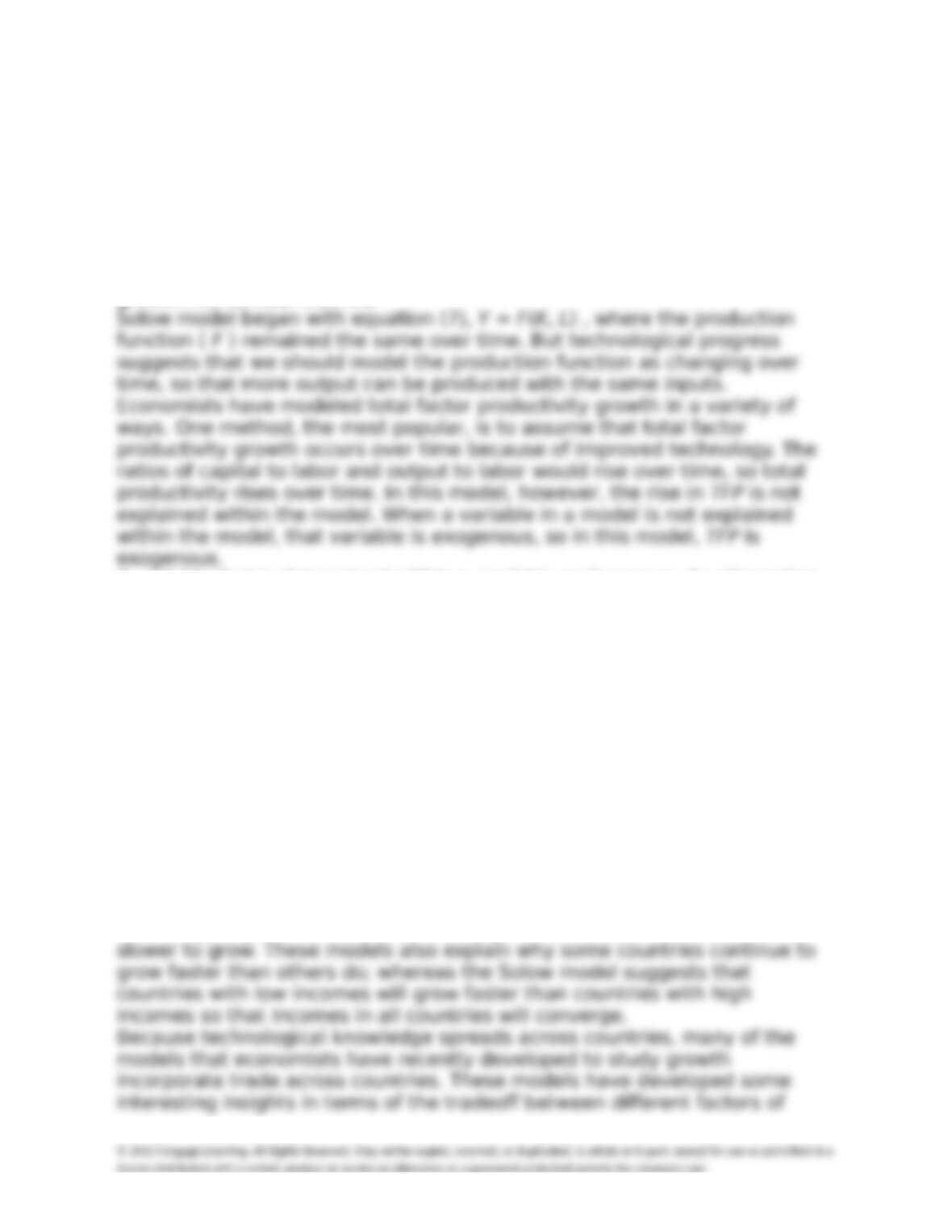
The answer is no, because of the possibility of total factor productivity
growth. Remember that the
A variable that is determined within a model is endogenous. An alternative
model, called an endogenous-growth model, seeks to explain how total
factor productivity grows, rather than simply assuming that it does so
exogenously. Productivity does not just materialize from nothing, but results
from investments that people and companies make in new technology,
through research and development. It results from knowledge and creative
endeavors. It comes about because people, .rms, and governments spend
resources exploring the unknown. Endogenous-growth models try to explain
some of the possible avenues through which productivity growth occurs.
They also examine the consequences for such growth on the economy.
One prediction of endogenous-growth models is that the world’s leader in
technology may grow faster than other countries. Economists have
struggled to explain why countries with similar characteristics (growth rate
of labor, depreciation rate, and savings rate) grow at diHerent rates. For
that reason, economists sometimes model how technology is adopted in
diHerent countries. Countries that are better able to develop new
technologies get an initial burst in their growth, while those that follow are
Chapter 10: Economic Growth and Business Cycles 113
production. For example, rapid growth in Asian countries such as Singapore
and Indonesia occurred in the 1980s and 1990s in large part because they
were better able to harness new technologies and develop them for use in
consumer and business products. In addition, they invested a huge amount
in physical capital. The result was economic growth that far exceeded the
growth rates of the major industrialized countries, enabling the Asian
countries to catch up substantially in terms of income.
ADDITIONAL QUESTIONS
1. Suppose the labor force is growing at a rate of 2 percent (so λ = 0.02),
capital depreciates at a rate of 13 percent per year (δ = 0.13), and the
savings rate is 10 percent (σ = 0.10). The production function in terms of
output per worker is y = 7.5 k − 0.5 k2. Calculate the steady-state values
of capital per worker and output per worker. If the savings rate were only
5 percent, what would be the steady-state values of capital and output
per worker?
2. According to the Solow model, which economy will grow faster in steady
state, one with a high savings rate or one with a low savings rate? Which
economy will have a higher output per worker in the steady state?
Assume both economies have the same population growth rate of
workers and the same depreciation rate. Explain your answer using a
diagram.
REFERENCES
Solow, Robert. “A Contribution to the Theory of Economic Growth,”
Quarterly Journal of Economics, February 1956, pp. 65-94.
Symposium on New Growth Theory, Journal of Economic Perspectives 8,
(Winter 1994),
pp. 3-72.