152 ❖ Chapter 8 /Application: The Costs of Taxation
SOLUTIONS TO TEXT PROBLEMS:
Quick Quizzes
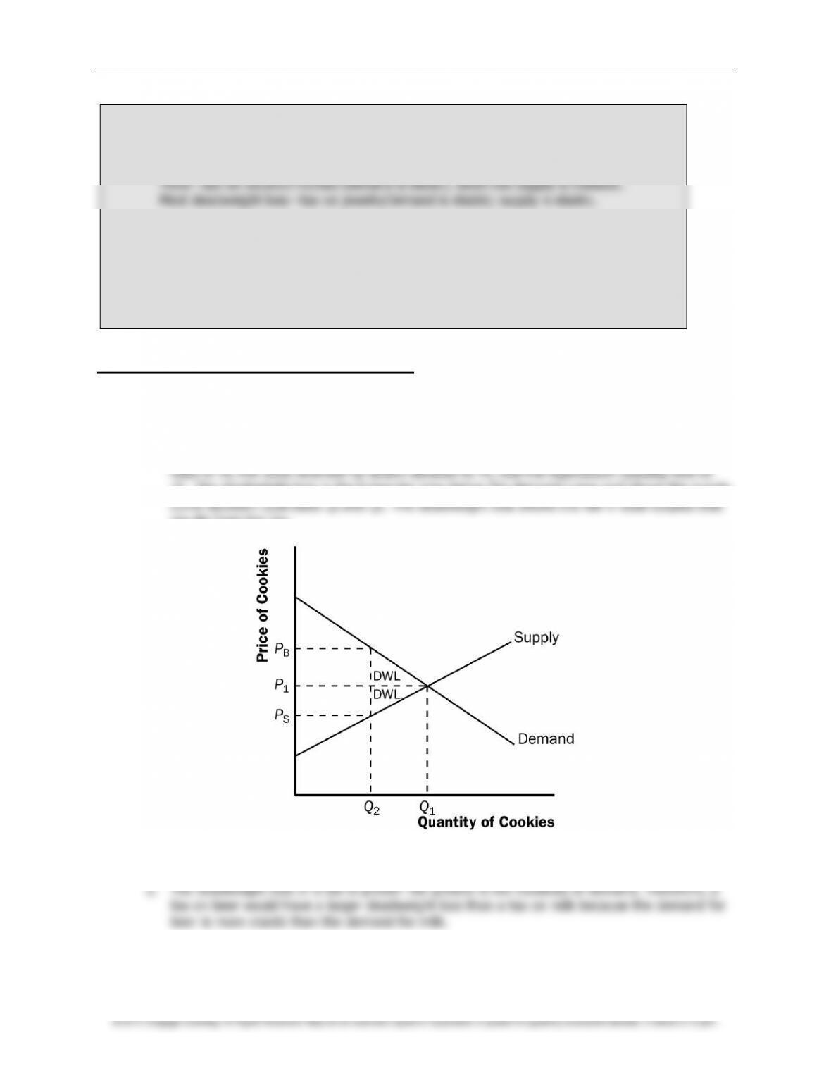
1. Figure 1 shows the supply and demand curves for cookies, with equilibrium quantity
Q
1 and
equilibrium price
P
1. When the government imposes a tax on cookies, the price to buyers
Q
2. The deadweight loss is the triangular area below the demand curve and above the supply
results from the tax.
Figure 1
B. Rank these taxes from smallest deadweight loss to largest deadweight loss.
Lowest deadweight loss—tax on children, very inelastic
Then—tax on food. Demand is inelastic; supply is elastic.
Third—tax on vacation homes Demand is elastic; short-run supply is inelastic.
Most deadweight loss—tax on jewelryDemand is elastic; supply is elastic.
C. Is deadweight loss the only thing to consider when designing a tax system?
No. This can generate a lively discussion. There are a variety of equity or fairness
concerns. The taxes on children and on food would be regressive. Each of the taxes
would tax certain households at much higher rates than other households with similar
incomes.
Chapter 8 /Application: The Costs of Taxation ❖ 153
3. If the government doubles the tax on gasoline, the revenue from the gasoline tax could rise
tax rate rises.
Questions for Review
1. When the sale of a good is taxed, both consumer surplus and producer surplus decline. The
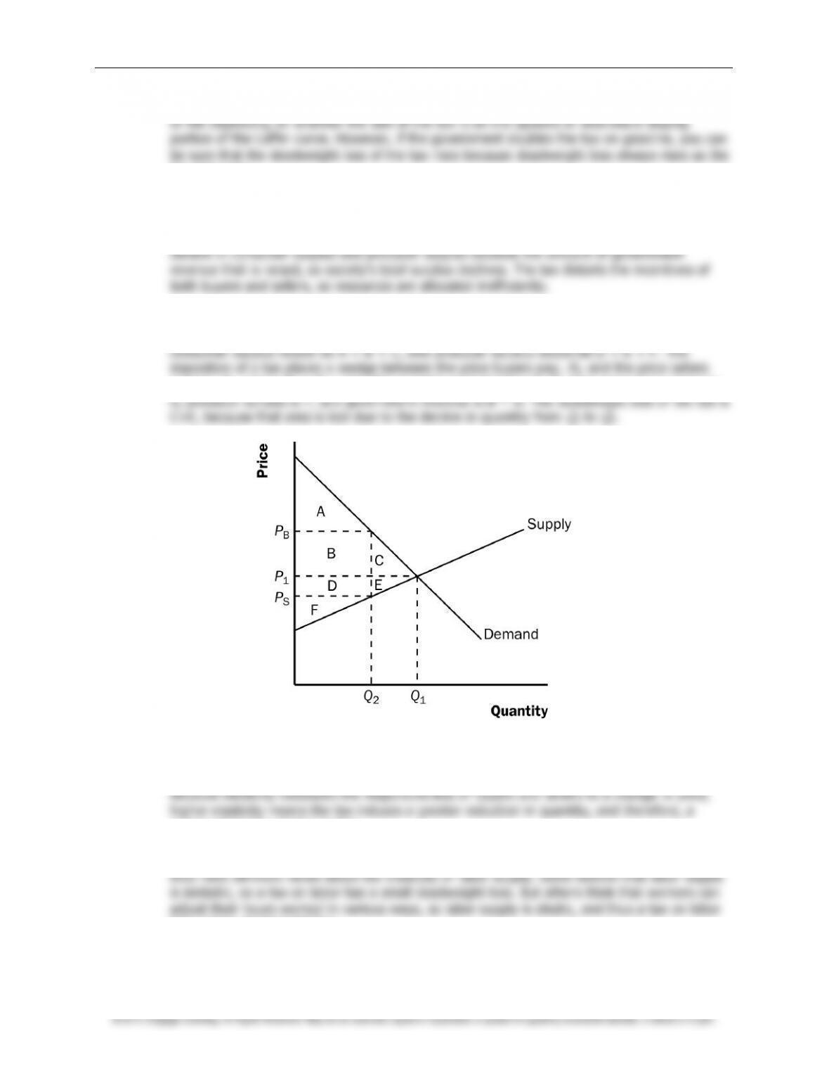
2. Figure 2 illustrates the deadweight loss and tax revenue from a tax on the sale of a good.
Without a tax, the equilibrium quantity would be
Q
1, the equilibrium price would be
P
1,
receive,
P
S, where
P
B =
P
S + tax. The quantity sold declines to
Q
2. Now consumer surplus is
Figure 2
3. The greater the elasticities of demand and supply, the greater the deadweight loss of a tax.
greater distortion to the market.
4. Experts disagree about whether labor taxes have small or large deadweight losses because
has a large deadweight loss.
154 ❖ Chapter 8 /Application: The Costs of Taxation
5. The deadweight loss of a tax rises more than proportionally as the tax rises. Tax revenue,
declines.
Quick Check Multiple Choice
1. a
2. b
3. c
4. a
5. b
6. a
Problems and Applications
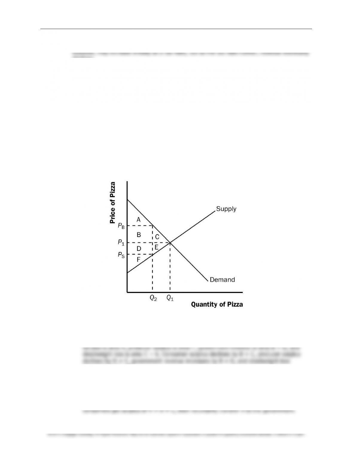
1. a. Figure 3 illustrates the market for pizza. The equilibrium price is
P
1, the equilibrium
quantity is
Q
1, consumer surplus is area A + B + C, and producer surplus is area D + E +
F. There is no deadweight loss, as all the potential gains from trade are realized; total
surplus is the entire area between the demand and supply curves: A + B + C + D + E +
F.
Figure 3
b. With a $1 tax on each pizza sold, the price paid by buyers,
P
B, is now higher than the
price received by sellers,
P
S, where
P
B =
P
S + $1. The quantity declines to
Q
2, consumer
increases by C + E.
c. If the tax were removed and consumers and producers voluntarily transferred B + D to
the government to make up for the lost tax revenue, then everyone would be better off
than without the tax. The equilibrium quantity would be
Q
1, as in the case without the
tax, and the equilibrium price would be
P
1. Consumer surplus would be A + C, because
Chapter 8 /Application: The Costs of Taxation ❖ 155
Producer surplus would be E + F, because producers get surplus of D + E + F, then
voluntarily transfer D to the government. Both consumers and producers are better off
than the case when the tax was imposed. If consumers and producers gave a little bit
2. a. The statement, “A tax that has no deadweight loss cannot raise any revenue for the
government,” is incorrect. An example is the case of a tax when either supply or demand
is perfectly inelastic. The tax has neither an effect on quantity nor any deadweight loss,
but it does raise revenue.
the quantity sold to zero.
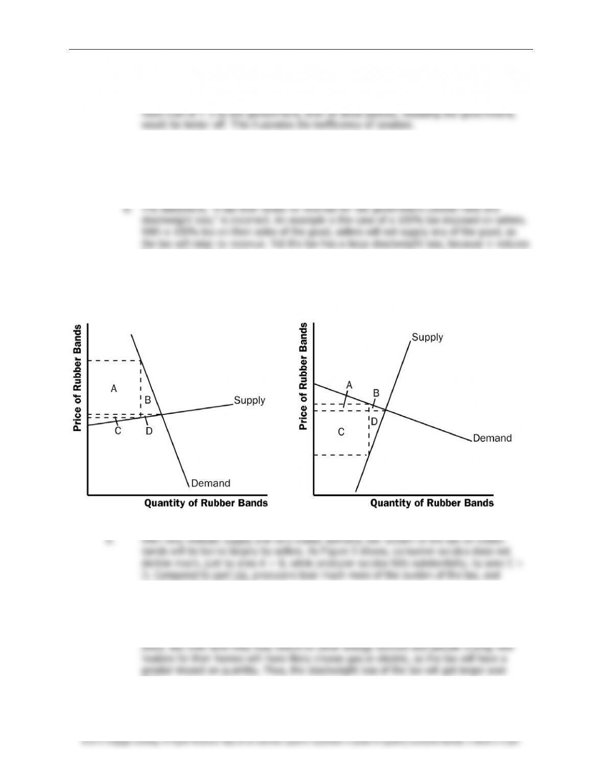
3. a. With very elastic supply and very inelastic demand, the burden of the tax on rubber
bands will be borne largely by buyers. As Figure 4 shows, consumer surplus declines
considerably, by area A + B, but producer surplus decreases only by area C+D..
Figure 4 Figure 5
consumers bear much less.
4. a. The deadweight loss from a tax on heating oil is likely to be greater in the fifth year after
it is imposed rather than the first year. In the first year, the demand for heating oil is
relatively inelastic, as people who own oil heaters are not likely to get rid of them right
time.
156 ❖ Chapter 8 /Application: The Costs of Taxation
b. The tax revenue is likely to be higher in the first year after it is imposed than in the fifth
5. Because the demand for food is inelastic, a tax on food is a good way to raise revenue
because it leads to a small deadweight loss; thus taxing food is less inefficient than taxing
other things. But it is not a good way to raise revenue from an equity point of view, because
poorer people spend a higher proportion of their income on food. The tax would affect them
more than it would affect wealthier people.
b. Senator Moynihan’s goal was probably to ban the use of hollow-tipped bullets. In this
case, the tax could be as effective as an outright ban.
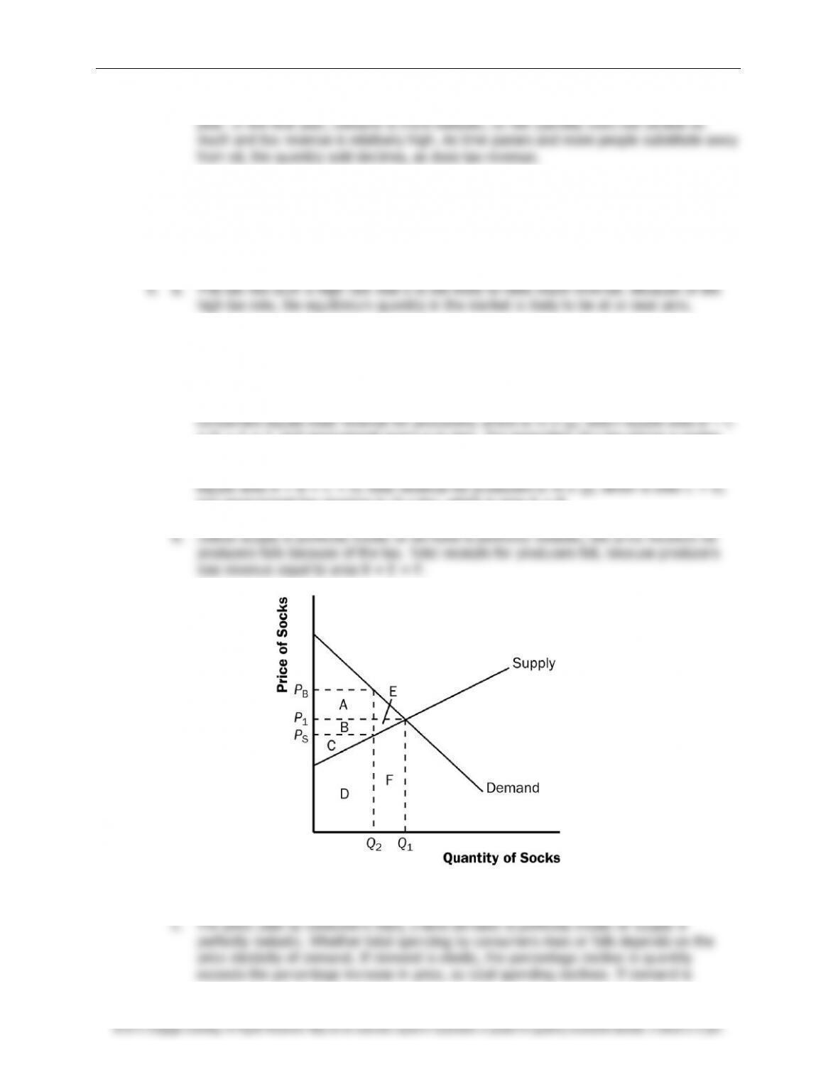
7. a. Figure 6 illustrates the market for socks and the effects of the tax. Without a tax, the
equilibrium quantity would be
Q
1, the equilibrium price would be
P
1, total spending by
+ D + E + F, and government revenue is zero. The imposition of a tax places a wedge
between the price buyers pay,
P
B, and the price sellers receive,
P
S, where
P
B =
P
S + tax.
The quantity sold declines to
Q
2. Now total spending by consumers is
P
B x
Q
2, which
and government tax revenue is
Q
2 x tax, which is area A + B.
Figure 6
Chapter 8 /Application: The Costs of Taxation ❖ 157
inelastic, the percentage decline in quantity is less than the percentage increase in price,
so total spending rises. Whether total consumer spending falls or rises, consumer surplus
declines because of the increase in price and reduction in quantity.
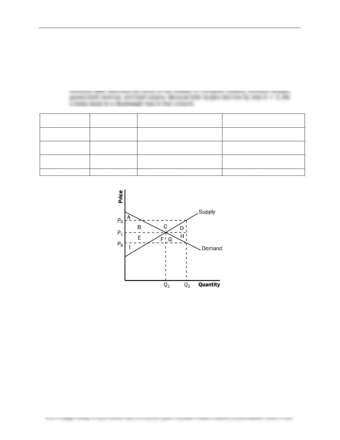
8. Figure 7 illustrates the effects of the $2 subsidy on a good. Without the subsidy, the
equilibrium price is
P
1 and the equilibrium quantity is
Q
1. With the subsidy, buyers pay price
P
B, producers receive price
P
S (where
P
S =
P
B + $2), and the quantity sold is
Q
2. The
Before
Subsidy
After Subsidy
Change
Consumer
Surplus
A + B
A + B + E + F + G
+(E + F + G)
Producer
Surplus
E + I
B + C + E + I
+(B + C)
Government
Revenue
0
–(B + C + D + E + F + G + H)
–(B + C + D + E + F + G + H)
Total Surplus
A + B + E + I
A + B – D + E – H + I
–(D + H)
Figure 7
158 ❖ Chapter 8 /Application: The Costs of Taxation
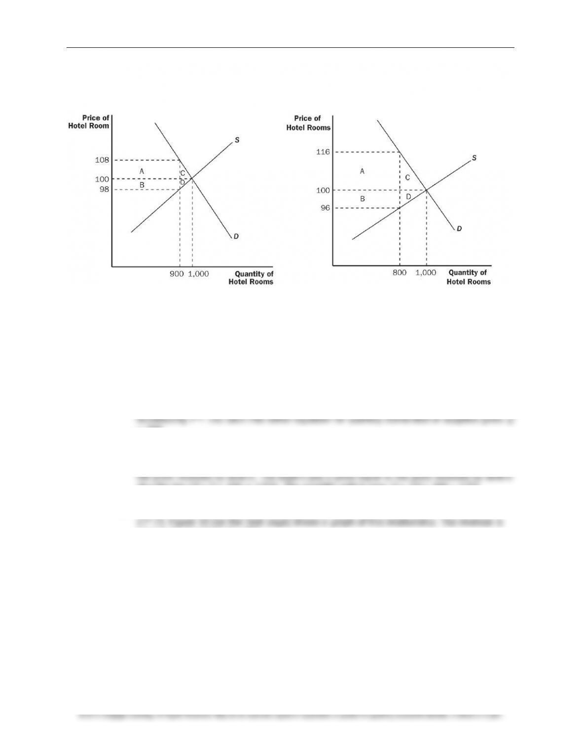
9. a. Figure 8 shows the effect of a $10 tax on hotel rooms. The tax revenue is represented by
areas A + B, which are equal to ($10)(900) = $9,000. The deadweight loss from the tax
is represented by areas C + D, which are equal to (0.5)($10)(100) = $500.
Figure 8 Figure 9
b. Figure 9 shows the effect of a $20 tax on hotel rooms. The tax revenue is represented by
areas A + B, which are equal to ($20)(800) = $16,000. The deadweight loss from the tax
is represented by areas C + D, which are equal to (0.5)($20)(200) = $2,000.
When the tax is doubled, the tax revenue rises by less than double, while the deadweight
loss rises by more than double. The higher tax creates a greater distortion to the market.
10. a. Setting quantity supplied equal to quantity demanded gives 2
P
= 300 –
P
. Adding
P
to
both sides of the equation gives 3
P
= 300. Dividing both sides by 3 gives
P
= 100.
= 200.
b. Now P is the price received by sellers and
P
+
T
is the price paid by buyers. Equating
quantity demanded to quantity supplied gives
2P
= 300 − (
P
+
T
). Adding
P
to both sides
of the equation gives 3
P
= 300 –
T
. Dividing both sides by 3 gives
P
= 100 –
T
/3. This is
plus the tax (
P
+
T
= 100 + 2
T
/3). The quantity sold is now
Q
= 2
P
= 200 – 2
T
/3.
c. Because tax revenue is equal to
T
x
Q
and
Q
= 200 – 2
T
/3, tax revenue equals 200
T
−
2
T
zero at
T
= 0 and at
T
= 300.
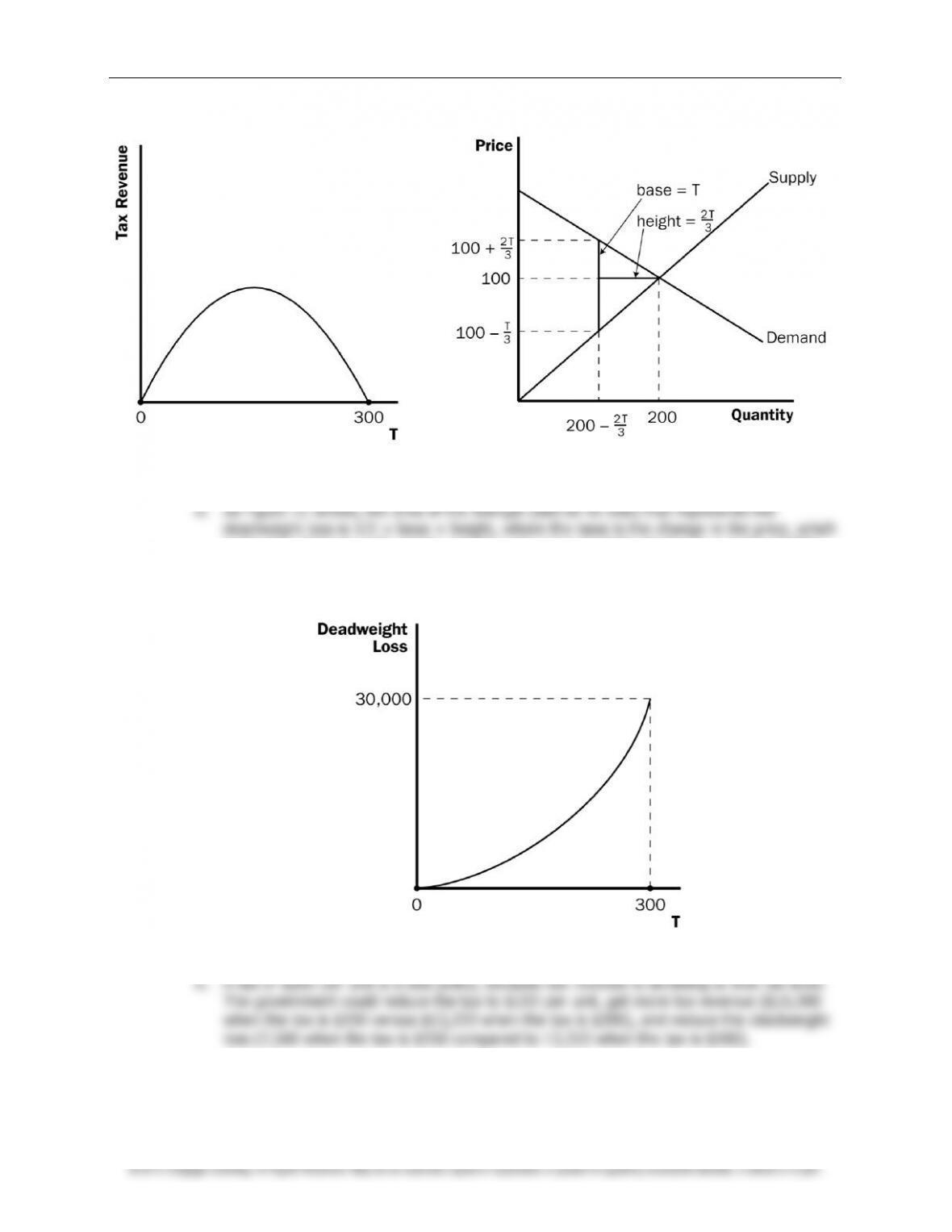
Chapter 8 /Application: The Costs of Taxation ❖ 159
Figure 10 Figure 11
is the size of the tax (
T
) and the height is the amount of the decline in quantity (2
T
/3).
So the deadweight loss equals 1/2 ×
T
× 2
T
/3 =
T
2/3. This rises exponentially from 0
(when
T
= 0) to 30,000 when
T
= 300, as shown in Figure 12.
Figure 12