Chapter 7/Consumers, Producers, and the Efficiency of Markets ❖ 131
Figure 3
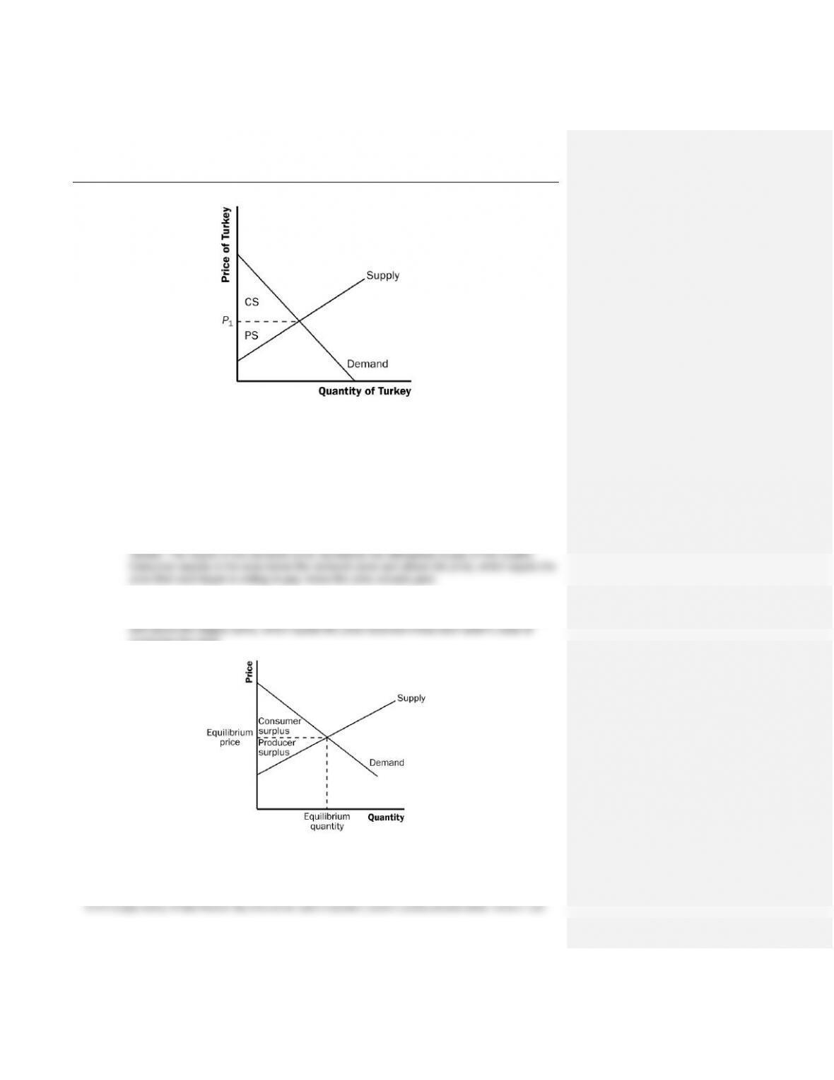
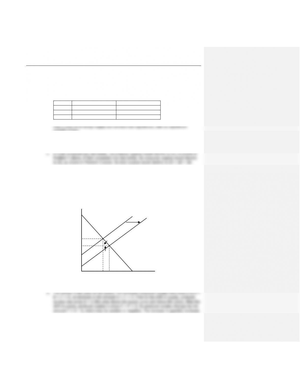
3. Figure 3 shows the supply and demand for turkey. The price of turkey is
P
1, consumer
surplus is CS, and producer surplus is PS. Producing more turkeys than the equilibrium
quantity would lower total surplus because the value to the marginal buyer would be lower
than the cost to the marginal seller on those additional units.
Questions for Review
1. The price a buyer is willing to pay, consumer surplus, and the demand curve are all closely
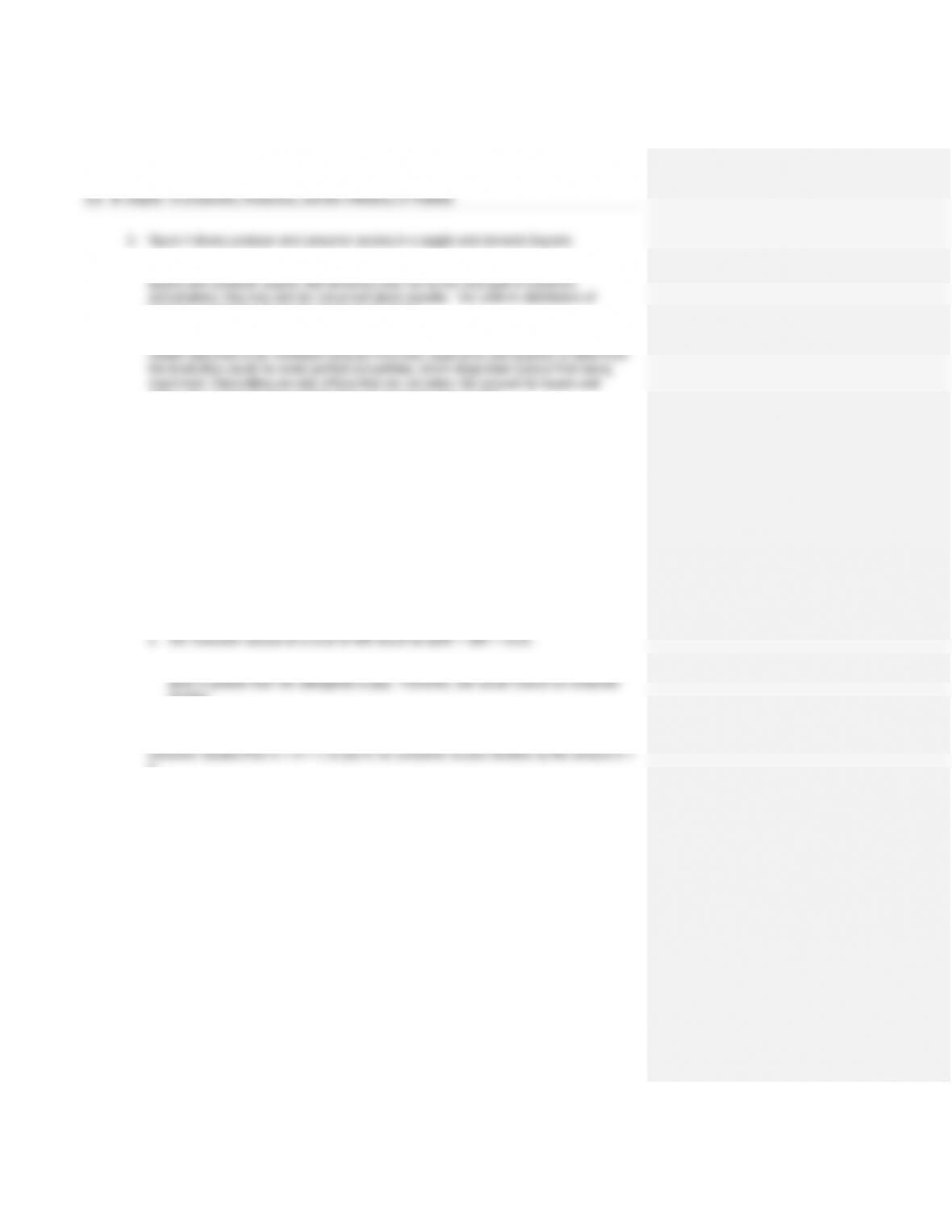
2. Sellers’ costs, producer surplus, and the supply curve are all closely related. The height of the
supply curve represents the costs of the sellers. Producer surplus is the area below the price
producing the good.
Figure 4
© 2012 Cengage Learning. All Rights Reserved. May not be scanned, copied or duplicated, or posted to a publicly accessible website, in whole or in part.
4. An allocation of resources is efficient if it maximizes total surplus, the sum of consumer
economic prosperity among the members of society.
5. Two types of market failure are market power and externalities. Market power may cause
sellers. As a result, the free market does not maximize total surplus.
Quick Check Multiple Choice
1. a
2. a
3. b
4. c
5. b
6. c
Problems and Applications
1. a. Consumer surplus is equal to willingness to pay minus the price paid. Therefore,
Melissa’s willingness to pay must be $200 ($120 + $80).
c. If the price of an iPhone was $250, Melissa would not have purchased one because the
surplus.
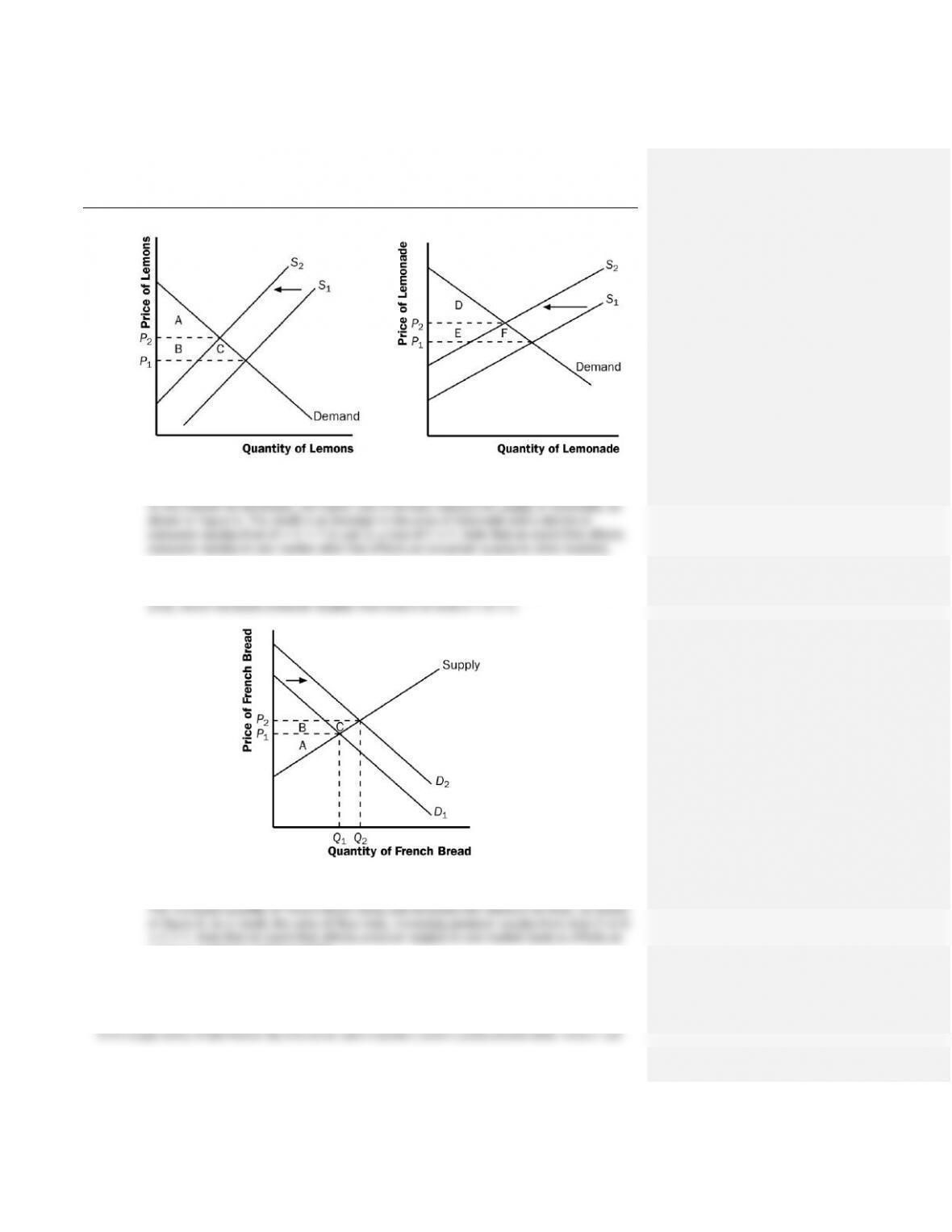
2. If an early freeze in California sours the lemon crop, the supply curve for lemons shifts to the
left, as shown in Figure 5. The result is a rise in the price of lemons and a decline in
C.
Chapter 7/Consumers, Producers, and the Efficiency of Markets ❖ 133
Figure 5 Figure 6
3. A rise in the demand for French bread leads to an increase in producer surplus in the market
for French bread, as shown in Figure 7. The shift of the demand curve leads to an increased
Figure 7
producer surplus in related markets.
© 2012 Cengage Learning. All Rights Reserved. May not be scanned, copied or duplicated, or posted to a publicly accessible website, in whole or in part.
consumer surplus is $3 + $1 = $4, which is the area of A in the figure.
c. When the price of each bottle of water falls from $4 to $2, Bert buys three bottles of
water, an increase of one. His consumer surplus consists of both areas A and B in the
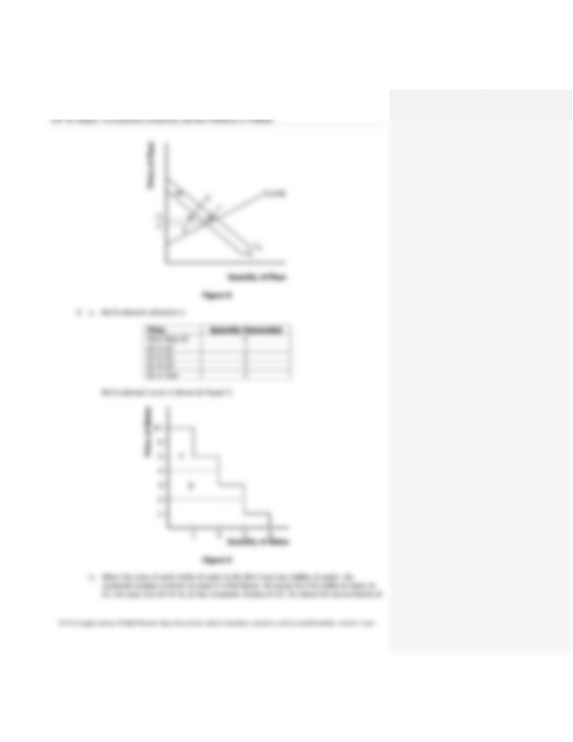
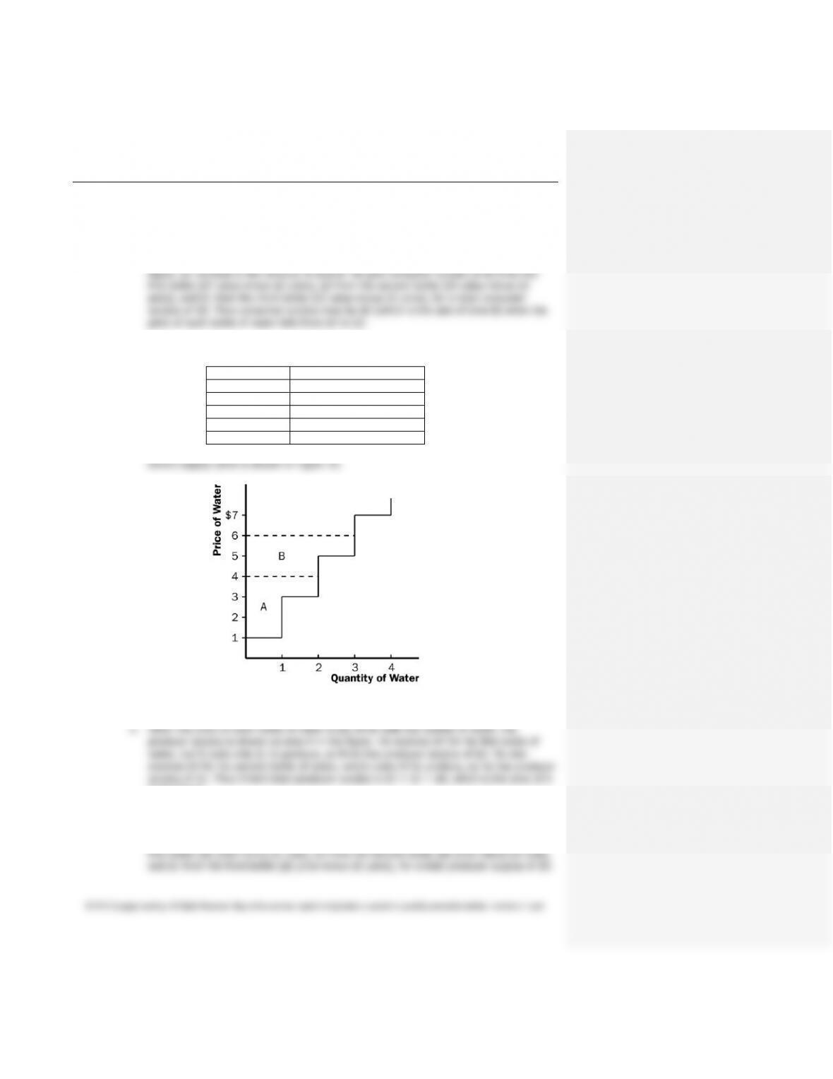
5. a. Ernie’s supply schedule for water is:
Price
Quantity Supplied
More than $7
4
$5 to $7
3
$3 to $5
2
$1 to $3
1
Less than $1
0
Figure 10
in the figure.
c. When the price of each bottle of water rises from $4 to $6, Ernie sells three bottles of
water, an increase of one. His producer surplus consists of both areas A and B in the
figure, an increase by the amount of area B. He gets producer surplus of $5 from the
© 2012 Cengage Learning. All Rights Reserved. May not be scanned, copied or duplicated, or posted to a publicly accessible website, in whole or in part.
bottle of water rises from $4 to $6.
6. a. From Ernie’s supply schedule and Bert’s demand schedule, the quantity demanded and
supplied are:
Price
Quantity Supplied
Quantity Demanded
$2
1
3
$4
2
2
$6
3
1
quantity of two.
b. At a price of $4, consumer surplus is $4 and producer surplus is $4, as shown in
Problems 3 and 4 above. Total surplus is $4 + $4 = $8.
d. If Ernie produced one additional bottle of water, his cost would be $5, but the price is
only $4, so his producer surplus would decline by $1. If Bert consumed one additional
bottle of water, his value would be $3, but the price is $4, so his consumer surplus would
decline by $1. So total surplus declines by $1 + $1 = $2.
7. a. The effect of falling production costs in the market for flat-screen TVs results in a shift to
the right in the supply curve, as shown in Figure 11. As a result, the equilibrium price of
flat-screen TVs declines and the equilibrium quantity increases.
Figure 11
Price of flat-screen
TVs
Quantity of flat-screen TVs
Demand
S2
S1
P
1
P
2
Q
1
Q
2
E
A
B
F
C
G
D