Chapter 18/The Markets for the Factors of Production ❖ 331
Figure 1
4. The income of the owners of land and capital is determined by the value of the marginal
contribution of land and capital to the production process.
An increase in the quantity of capital would reduce the marginal product of capital, thus
reducing the incomes of those who already own capital. However, it would increase the
incomes of workers because a higher capital stock raises the marginal product of labor.
Questions for Review
1. A firm’s production function describes the relationship between the quantity of labor used in
production and the quantity of output from production. The marginal product of labor is the
A competitive, profit-maximizing firm hires workers up to the point where the value of the
marginal product of labor equals the wage. As a result, the value–of-marginal-product curve
is the firm’s labor-demand curve.
2. Events that could shift the demand for labor include changes in the output price,
product of labor, which in turn increases the demand for labor and shifts the labor-demand
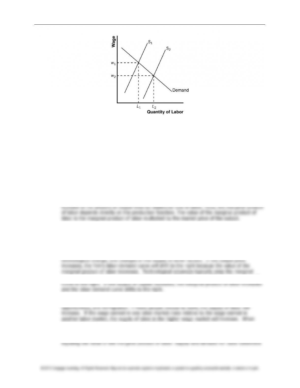
3. Events that could shift the supply of labor include changes in tastes, changes in alternative
immigrants enter a country, the supply of labor in that country increases.
4. The wage can adjust to balance the supply and demand for labor while simultaneously
© 2012 Cengage Learning. All Rights Reserved. May not be scanned, copied or duplicated, or posted to a publicly accessible website, in whole or in part.
the equilibrium wage. Firms maximize profits by choosing the amount of labor where the
wage is equal to the value of the marginal product of labor.
5. A large wave of immigration would increase the supply of labor, thus reducing the wage.
Quick Check Multiple Choice
1. c
2. b
3. a
4. b
5. d
6. d
Problems and Applications
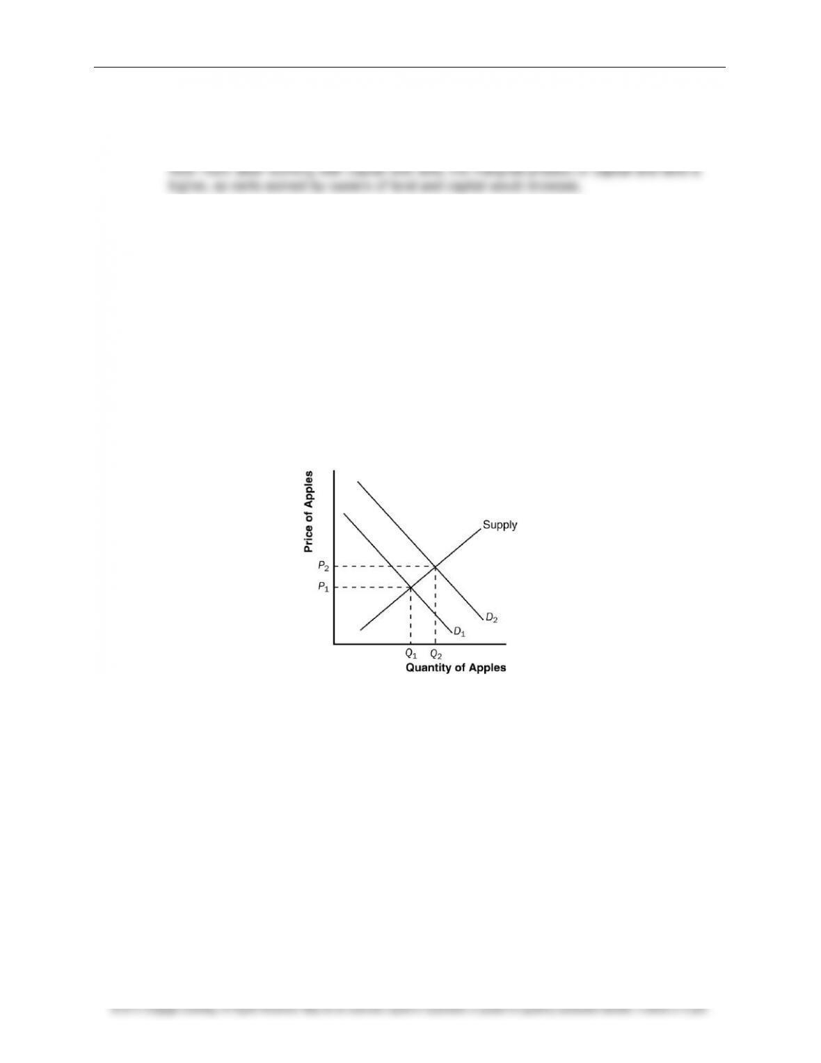
1. a. The law requiring people to eat one apple a day increases the demand for apples. As
shown in Figure 2, demand shifts from
D
1 to
D
2, increasing the price from
P
1 to
P
2, and
increasing quantity from
Q
1 to
Q
2.
Figure 2
b. Because the price of apples increases, the value of the marginal product increases for
any given quantity of labor. There is no change in the marginal product of labor for any
given quantity of labor. However, firms will choose to hire more workers and thus the
marginal product of labor at the profit-maximizing level of labor will be lower.
c. As Figure 3 shows, the increase in the value of the marginal product of labor shifts the
demand curve of labor from
D
1 to
D
2. The equilibrium quantity of labor rises from
L
1 to
L
2, and the wage rises from
w
1 to
w
2.
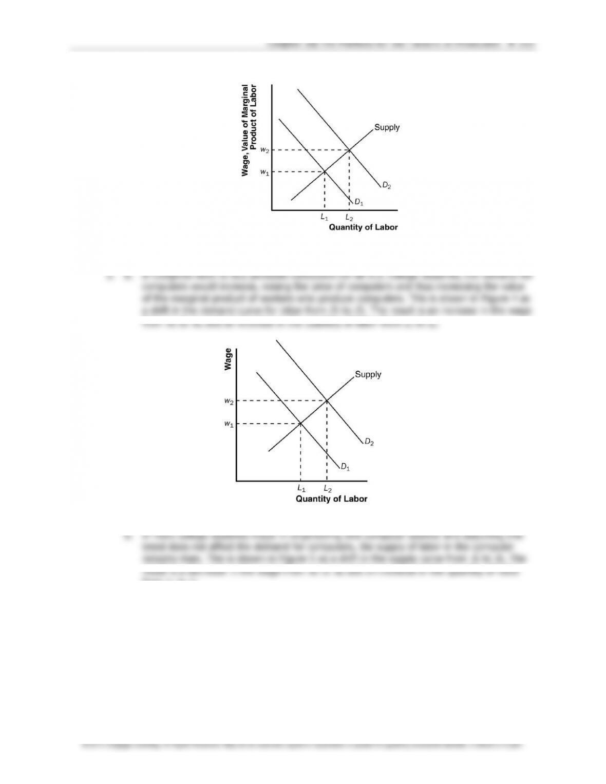
Figure 3
Figure 4
from
L
1 to
L
2.
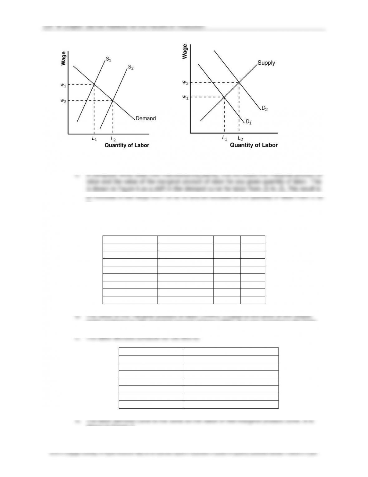
Figure 5 Figure 6
L
2.
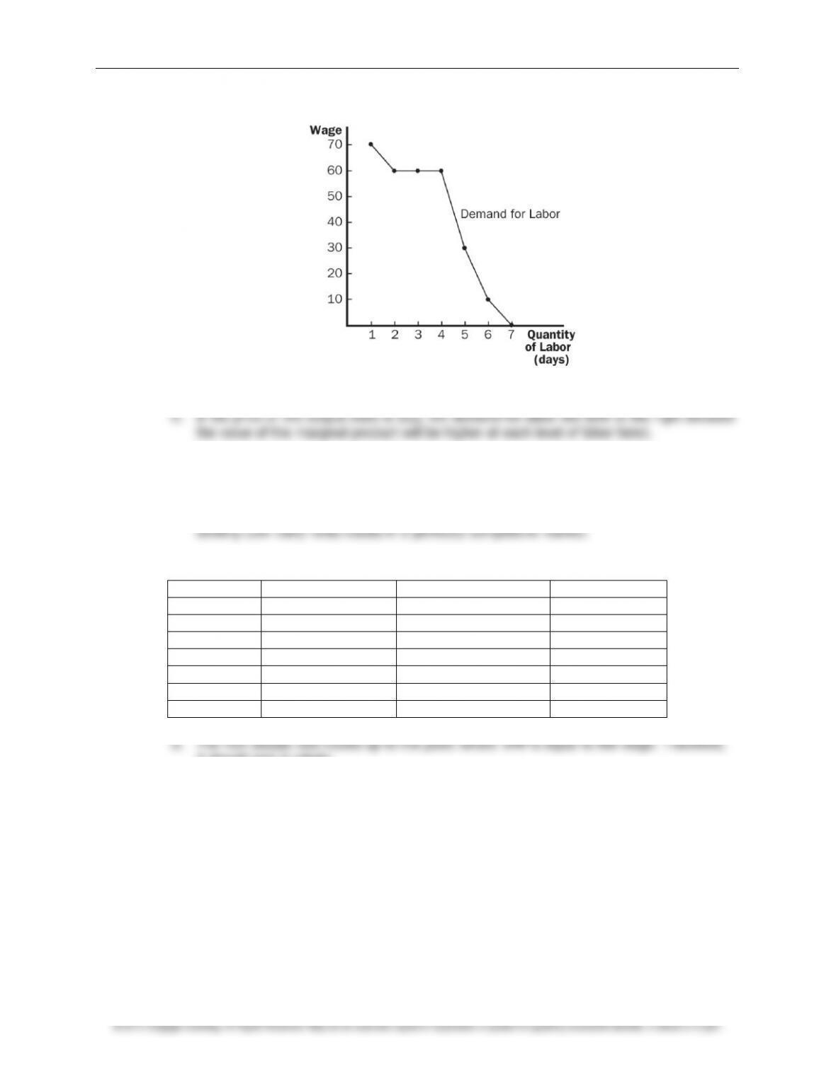
3. a. The marginal product of labor is equal to the additional output produced by an additional
unit of labor. The table below shows the marginal product of labor (
MPL
) for this firm:
Days of Labor
Units of Output
MPL
VMPL
0
0
—
—
1
7
7
70
2
13
6
60
3
19
6
60
4
25
6
60
5
28
3
30
6
29
1
10
7
29
0
0
($10) multiplied by the marginal product of labor (
MPL
). It is also reported in the table.
Wage
Quantity of Labor Demanded
$0
7
10
6
30
5
60
4
60
3
60
2
70
1
shown in Figure 7.
Chapter 18/The Markets for the Factors of Production ❖ 335
Figure 7
4. a. Because the firm can sell all of the milk it wants to at the market price of $4 per gallon,
Smiling Cow Dairy operates in a perfectly competitive output market.
b. Because the firm can rent all the robots it wants to at the market price of $100 per day,
c. The table below shows the
MP
and
VMP
for robots:
# Robots
Total Output
MP
VMP
0
0 gallons
—-
—-
1
50
50 gallons
$ 200
2
85
35
140
3
115
30
120
4
140
25
100
5
150
10
40
6
155
5
20
it should rent 4 robots.
5. a. The firm’s demand for labor is the same as its value of the marginal product. The firm will
set wage equal to
VMP
:
w
=
VMP
=
P
MPL
= 2(100 – 2
L
) = 200 – 4
L
The market demand curve for labor will be the horizontal summation of the 20 firm demand
curves (summed across
L
).
Rearranging the firm’s demand, we get
L
= 50 – 0.25
w
. Thus, the market demand curve
must be
L
= 20(50 – 0.25
w
) = 1,000 – 5
w.
b. If labor supply is inelastic at 200, then we can solve for wage by determining the market
equilibrium:
200 = 1,000 – 5
w
w
= 160.
900 apples. Total revenue for each firm will be (2)(900) = 1,800. Assuming that wages are
the firm’s only costs, total costs will be (160)(10) = 1,600, leaving each firm with profit =
200. Total income for the country will be (200)(160) + (20)(200) = 36,000.
firm’s demand for labor) rises.
w
=
VMP
=
P
MPL
= 4(100 – 2
L
) = 400 – 8
L
Rearranging for
L
, we get
L
= 50 – 0.125
w
. Thus, the market demand for labor becomes:
L
= 20(50 – 0.125
w
) = 1,000 – 2.5
w
. Finding the new equilibrium wage, we get:
200 = 1,000 – 2.5
w
w
= 320
Total income will be (320)(200) + (400)(20) = 72,000.
d. Now there are 10 orchards, so the market demand is 10 times the individual firm demand
curves:
L
= 10(50 – 0.25
w
) = 500 – 2.5
w
. Solving for the equilibrium wage, we get:
200 = 500 – 2.5
w
w
= 120
Total revenue = (2)(1,600) = 3,200
Total cost = (120)(20) = 2,400. So profit = 800.
fallen in the country.
6. Because your uncle is maximizing his profit, he must be hiring workers such that their wage
the marginal product of a worker must be two sandwiches per hour.
7. a. Leadbelly should hire workers up to the point where
VMP
is equal to the wage of $150
per day.

c. As Figure 8 shows, the market wage is determined in the labor market ($150 per day).
The firm takes this wage as given and chooses its level of labor where
VMP
is equal to
$150 per day.
Figure 8
and a lower level of labor.
Figure 9
8. a. Figure 10 shows the U.S. capital market when there is an inflow of capital from abroad.
The inflow of capital shifts the supply curve to the right, from
S
1 to
S
2. The result is a
capital from
K
1 to
K
2.

Figure 10
in the demand for labor from
D
1 to
D
2. As a result, the wage rate rises from
w
1 to
w
2 and
the quantity of labor rises from
L
1 to
L
2.
Figure 11
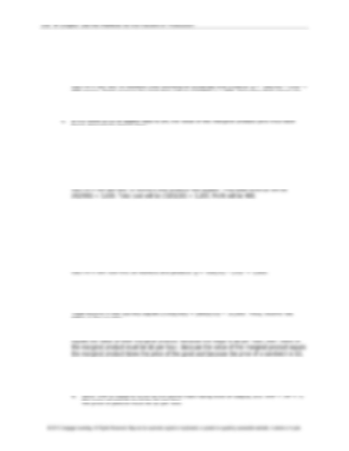
9. a. If a firm already gives workers fringe benefits valued at more than $3, the new law
would have no effect. But a firm that currently has fringe benefits less than $3 would be
affected by the law. Imagine a firm that currently pays no fringe benefits at all. The
requirement that it pay fringe benefits of $3 reduces the value of the marginal product of
labor effectively by $3 in terms of the cash wage the firm is willing to pay. This is shown
in Figure 12 as a leftward shift in the firm’s demand for labor from
D
1 to
D
2, a shift of
exactly $3.
Chapter 18/The Markets for the Factors of Production ❖ 339
Figure 12
of labor also declines.
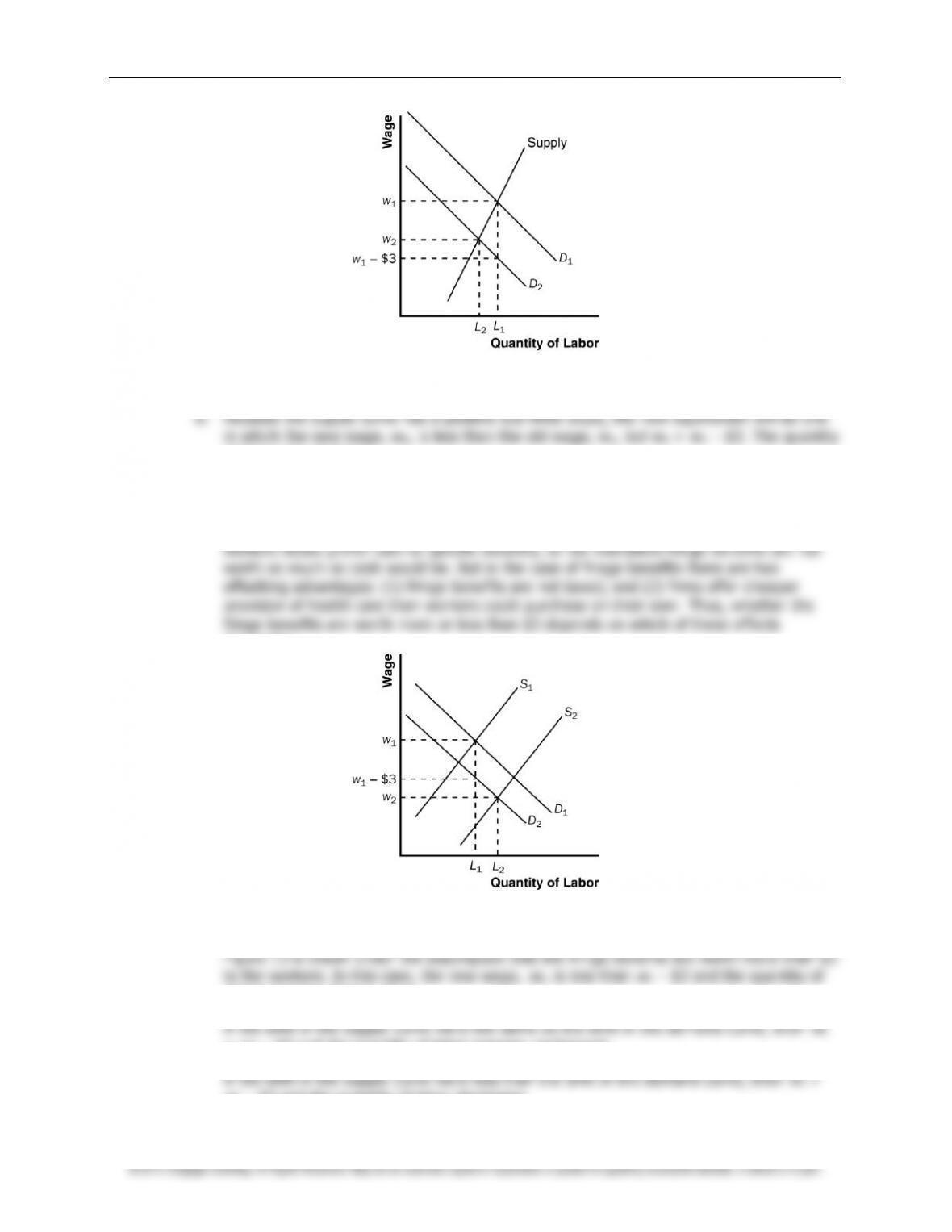
c. The preceding analysis is incomplete, of course, because it ignores the fact that the
fringe benefits are valuable to workers. As a result, the supply curve of labor might
increase, shown as a shift to the right in the supply of labor in Figure 13. In general,
dominates.
Figure 13
labor increases from
L
1 to
L
2.
=
w
1 – $3 and the quantity of labor remains unchanged.
w
1 – $3 and the quantity of labor decreases.

340 ❖ Chapter 18/The Markets for the Factors of Production
© 2012 Cengage Learning. All Rights Reserved. May not be scanned, copied or duplicated, or posted to a publicly accessible website, in whole or in part.
In all three cases, there is a lower wage and higher quantity of labor than if the supply
curve were unchanged.
d. Because a minimum-wage law would not allow the wage to decline when greater fringe
benefits are mandated, it would lead to increased unemployment, because firms would
refuse to pay workers more than the value of their marginal product.