Chapter 13/The Costs of Production ❖ 231
A. The division of total costs into fixed and variable costs will vary from firm to firm.
2. Once a factory is chosen, the firm must deal with the short-run costs associated with that
plant size.
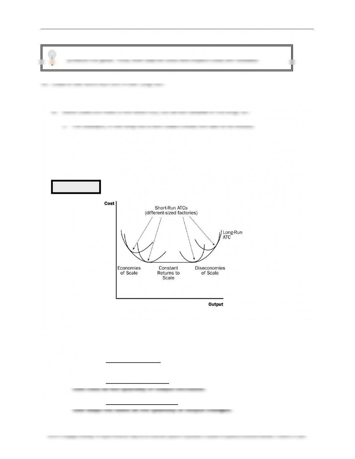
C. The long-run average-total-cost curve lies along the lowest points of the short-run average-total-
cost curves because the firm has more flexibility in the long run to deal with changes in
production.
D. The long-run average-total-cost curve is typically U-shaped, but is much flatter than a typical
short-run average-total-cost curve.
E. The length of time for a firm to get to the long run will depend on the firm involved.
F. Economies and Diseconomies of Scale
1. Definition of economies of scale: the property whereby long-run average total cost
falls as the quantity of output increases.
2. Definition of diseconomies of scale: the property whereby long-run average total
3. Definition of constant returns to scale: the property whereby long-run average total
Figure 6
Emphasize that these cost curves include ALL costs for the resources needed to
produce the good. Thus, both explicit costs and implicit costs are included.
232 ❖ Chapter 13/The Costs of Production
4.
FYI: Lessons from a Pin Factory
perform many different tasks.
b. The use of specialization allows firms to achieve economies of scale.
SOLUTIONS TO TEXT PROBLEMS:
Quick Quizzes
1. Farmer McDonald’s opportunity cost is $300, consisting of 10 hours of lessons at $20 an hour
an economic loss of $100 ($200 sales minus $300 opportunity cost).
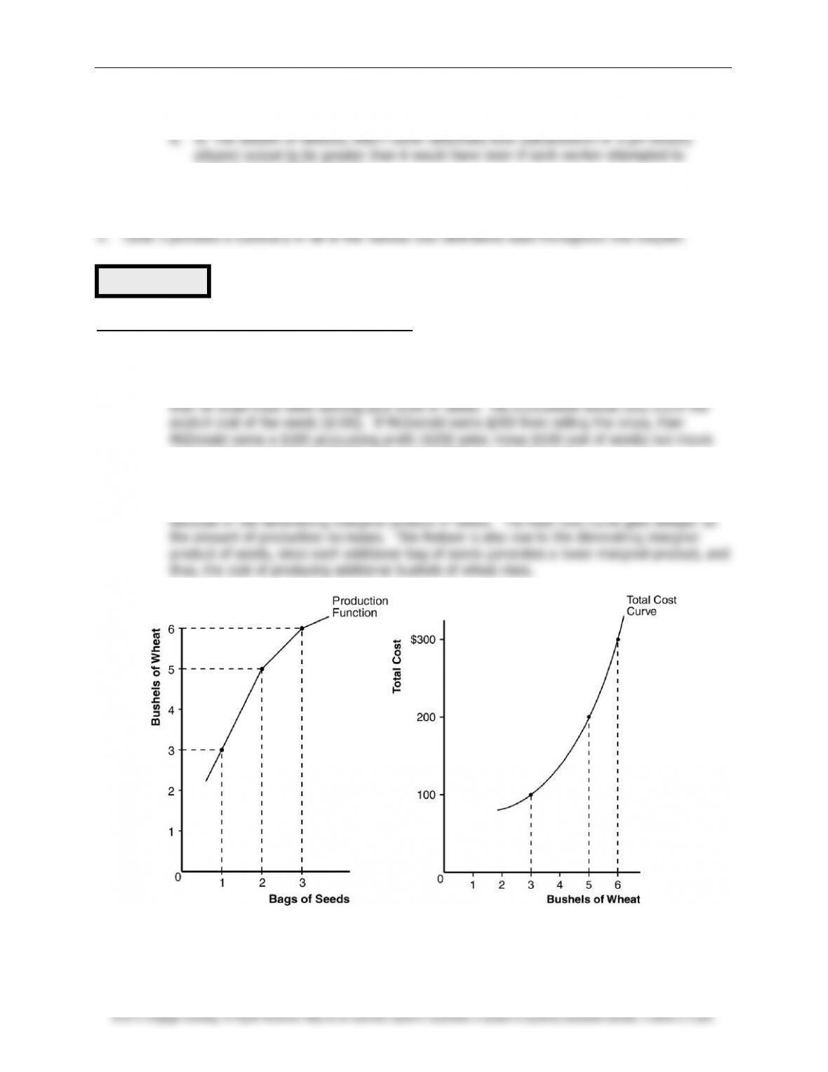
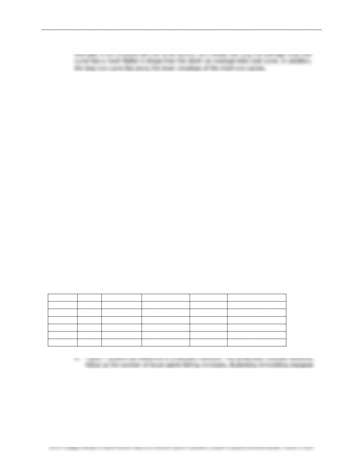
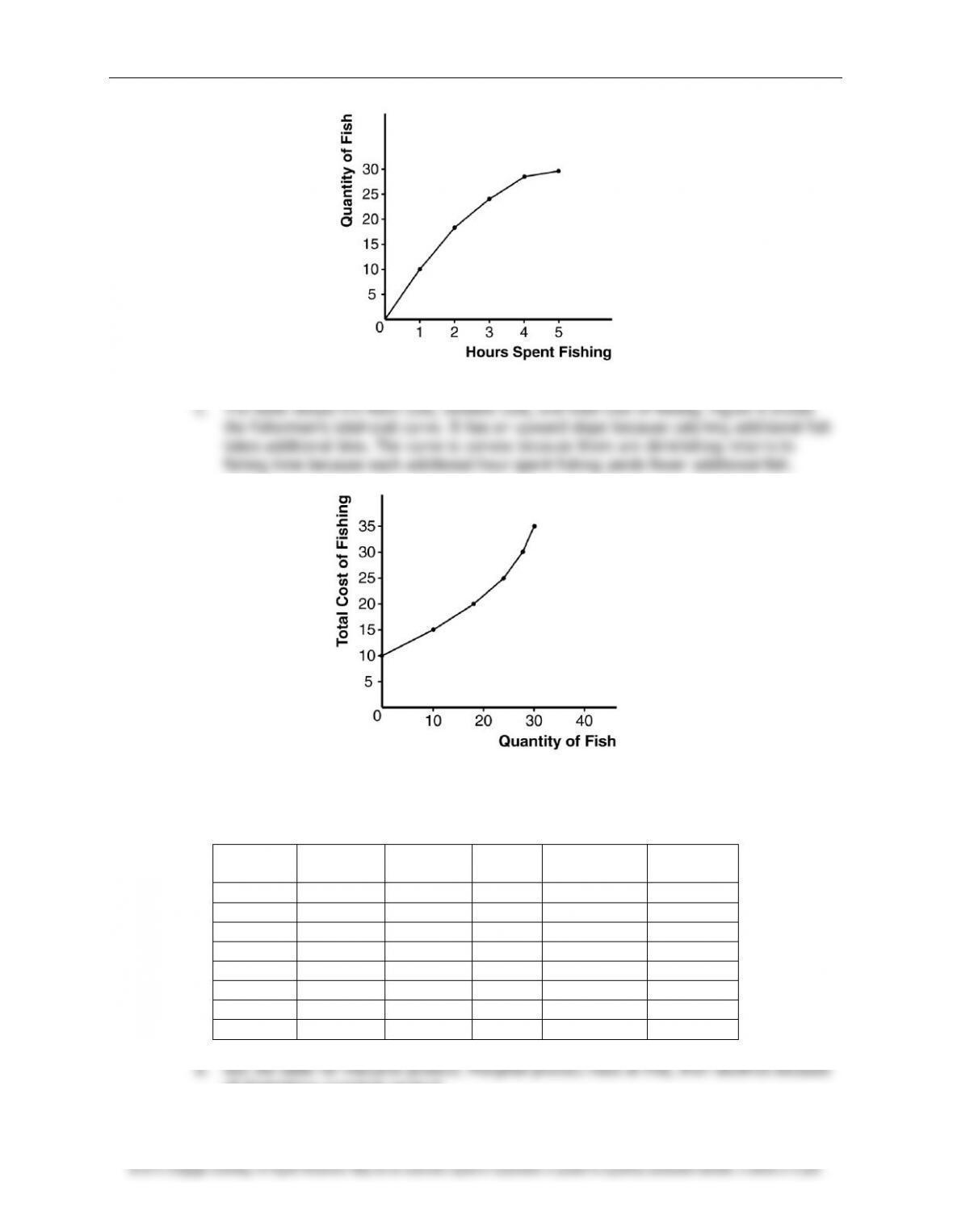
2. Farmer Jones’s production function is shown in Figure 1 and his total-cost curve is shown in
Figure 2. The production function becomes flatter as the number of bags of seeds increases
Figure 1 Figure 2
Table 3
Chapter 13/The Costs of Production ❖ 233
3. The average total cost of producing 5 cars is $250,000/5 = $50,000. Since total cost rose
from $225,000 to $250,000 when output increased from 4 to 5, the marginal cost of the fifth
car is $25,000.
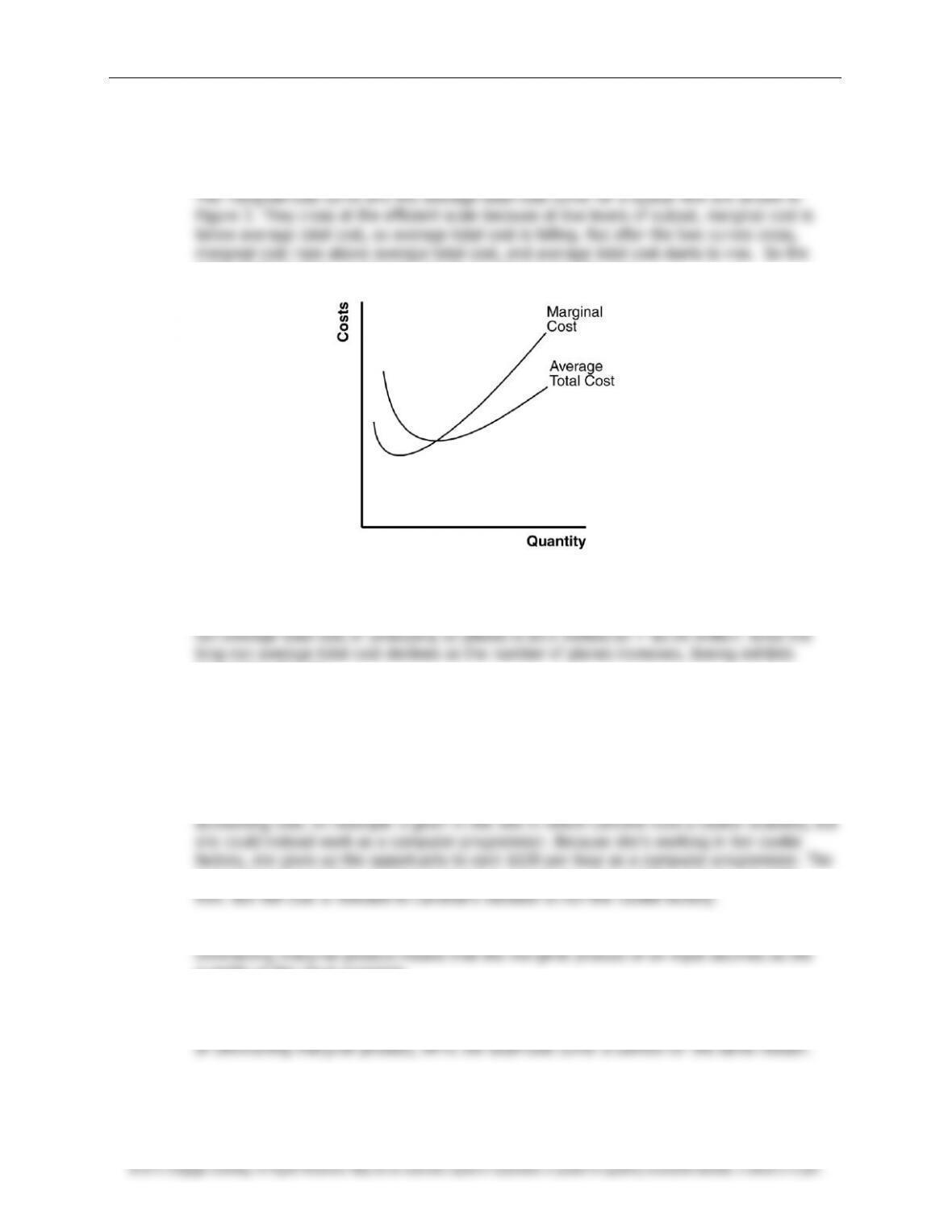
point of intersection must be the minimum of average total cost.
Figure 3
4. The long-run average total cost of producing 9 planes is $9 million/9 = $1 million. The long–
economies of scale.
Questions for Review
1. The relationship between a firm’s total revenue, profit, and total cost is profit equals total
revenue minus total costs.
2. An accountant would not count the owner’s opportunity cost of alternative employment as an
accountant ignores this opportunity cost because money does not flow into or out of the
3. Marginal product is the increase in output that arises from an additional unit of input.
quantity of the input increases.
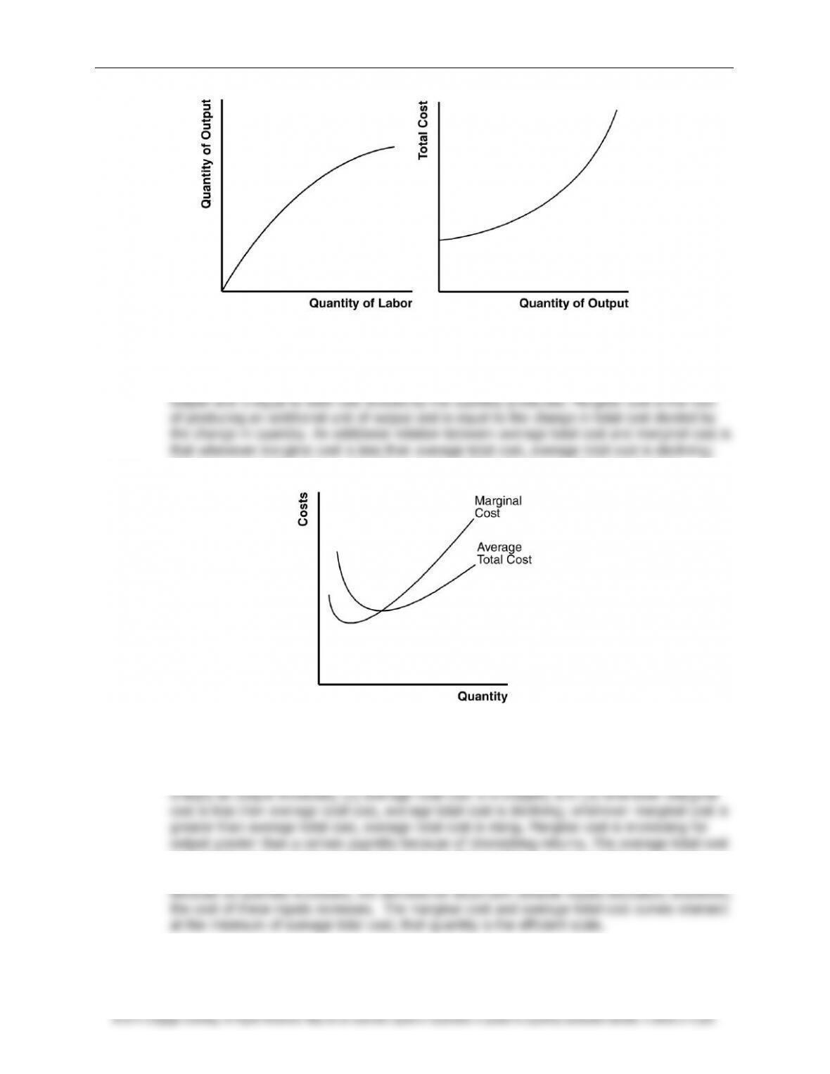
4. Figure 4 shows a production function that exhibits diminishing marginal product of labor.
Figure 5 shows the associated total-cost curve. The production function is concave because
234 ❖ Chapter 13/The Costs of Production
Figure 4 Figure 5
5. Total cost consists of the costs of all inputs needed to produce a given quantity of output. It
includes fixed costs and variable costs. Average total cost is the cost of a typical unit of
whenever marginal cost is greater than average total cost, average total cost is rising.
Figure 6
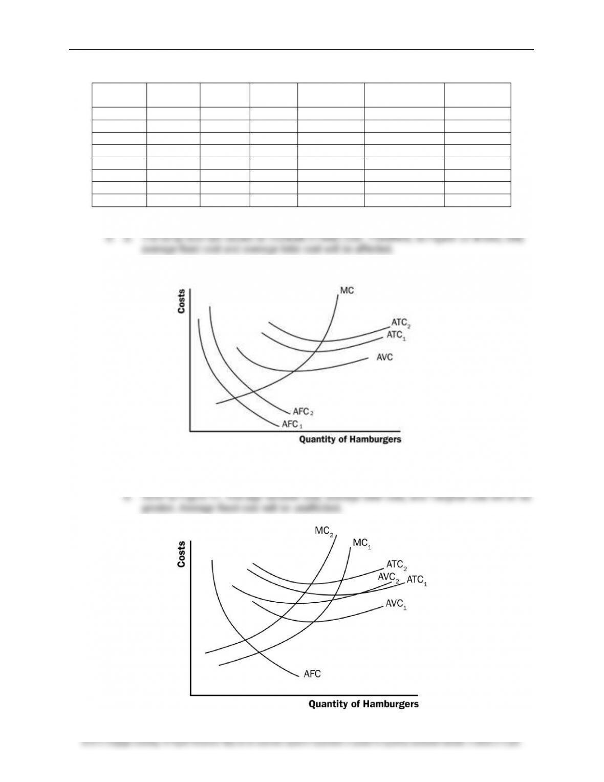
6. Figure 6 shows the marginal-cost curve and the average-total-cost curve for a typical firm.
There are three main features of these curves: (1) marginal cost is U-shaped but rises
curve is downward-sloping initially because the firm is able to spread out fixed costs over
additional units. The average-total-cost curve is increasing beyond some output level
Chapter 13/The Costs of Production ❖ 235
7. In the long run, a firm can adjust the factors of production that are fixed in the short run; for
8. Economies of scale exist when long-run average total cost decreases as the quantity of
output increases, which occurs because of specialization among workers. Diseconomies of
scale exist when long-run average total cost rises as the quantity of output increases, which
occurs because of the coordination problems inherent in a large organization.
Quick Check Multiple Choice
1. a
2. d
3. d
4. c
5. b
6. a
Problems and Applications
1. a. opportunity cost; b. average total cost; c. fixed cost; d. variable cost; e. total cost; f.
marginal cost.
2. a. The opportunity cost of something is what must be given up to acquire it.
b. The opportunity cost of running the hardware store is $550,000, consisting of $500,000
to rent the store and buy the stock and a $50,000 implicit cost, because your aunt would
quit her job as an accountant to run the store. Because the total opportunity cost of
$550,000 exceeds the projected revenue of $510,000, your aunt should not open the
store, as her economic profit would be negative.
3. a. The following table shows the marginal product of each hour spent fishing:
Hours
Fish
Fixed Cost
Variable Cost
Total Cost
Marginal Product
0
0
$10
$0
$10
—
1
10
10
5
15
10
2
18
10
10
20
8
3
24
10
15
25
6
4
28
10
20
30
4
5
30
10
25
35
2
product.
236 ❖ Chapter 13/The Costs of Production
Figure 7
Figure 8
4. Here is the completed table:
Workers
Output
Marginal
Product
Total
Cost
Average
Total Cost
Marginal
Cost
0
0
—
$200
—
—
1
20
20
300
$15.00
$5.00
2
50
30
400
8.00
3.33
3
90
40
500
5.56
2.50
4
120
30
600
5.00
3.33
5
140
20
700
5.00
5.00
6
150
10
800
5.33
10.00
7
155
5
900
5.81
20.00
of diminishing marginal product.
Chapter 13/The Costs of Production ❖ 237
b. See the table for total cost.
cost rises as quantity rises.
d. See the table for marginal cost. Marginal cost is also U-shaped, but rises steeply as
output increases. This is due to diminishing marginal product.
f. When marginal cost is less than average total cost, average total cost is falling; the cost
of the last unit produced pulls the average down. When marginal cost is greater than
average total cost, average total cost is rising; the cost of the last unit produced pushes
the average up.
6. a. The fixed cost is $300, because fixed cost equals total cost minus variable cost. At an
output of zero, the only costs are fixed cost.
b.
Quantity
Total
Cost
Variable
Cost
Marginal Cost
(using total cost)
Marginal Cost
(using variable cost)
0
$300
$0
—
—
1
350
50
$50
$50
2
390
90
40
40
3
420
120
30
30
4
450
150
30
30
5
490
190
40
40
6
540
240
50
50
7. The following table illustrates average fixed cost (
AFC
), average variable cost (
AVC
), and
because that minimizes average total cost.
238 ❖ Chapter 13/The Costs of Production
Quantity
Variable
Cost
Fixed
Cost
Total
Cost
Average
Fixed Cost
Average
Variable Cost
Average
Total Cost
0
$0.00
$200.00
$200.00
—
—
—
1
10.00
200.00
210.00
$200.00
$10.00
$210.00
2
20.00
200.00
220.00
100.00
10.00
110.00
3
40.00
200.00
240.00
66.67
13.33
80.00
4
80.00
200.00
280.00
50.00
20.00
70.00
5
160.00
200.00
360.00
40.00
32.00
72.00
6
320.00
200.00
520.00
33.33
53.33
86.67
7
640.00
200.00
840.00
28.57
91.43
120.00
Figure 10
Chapter 13/The Costs of Production ❖ 239
Figure 11
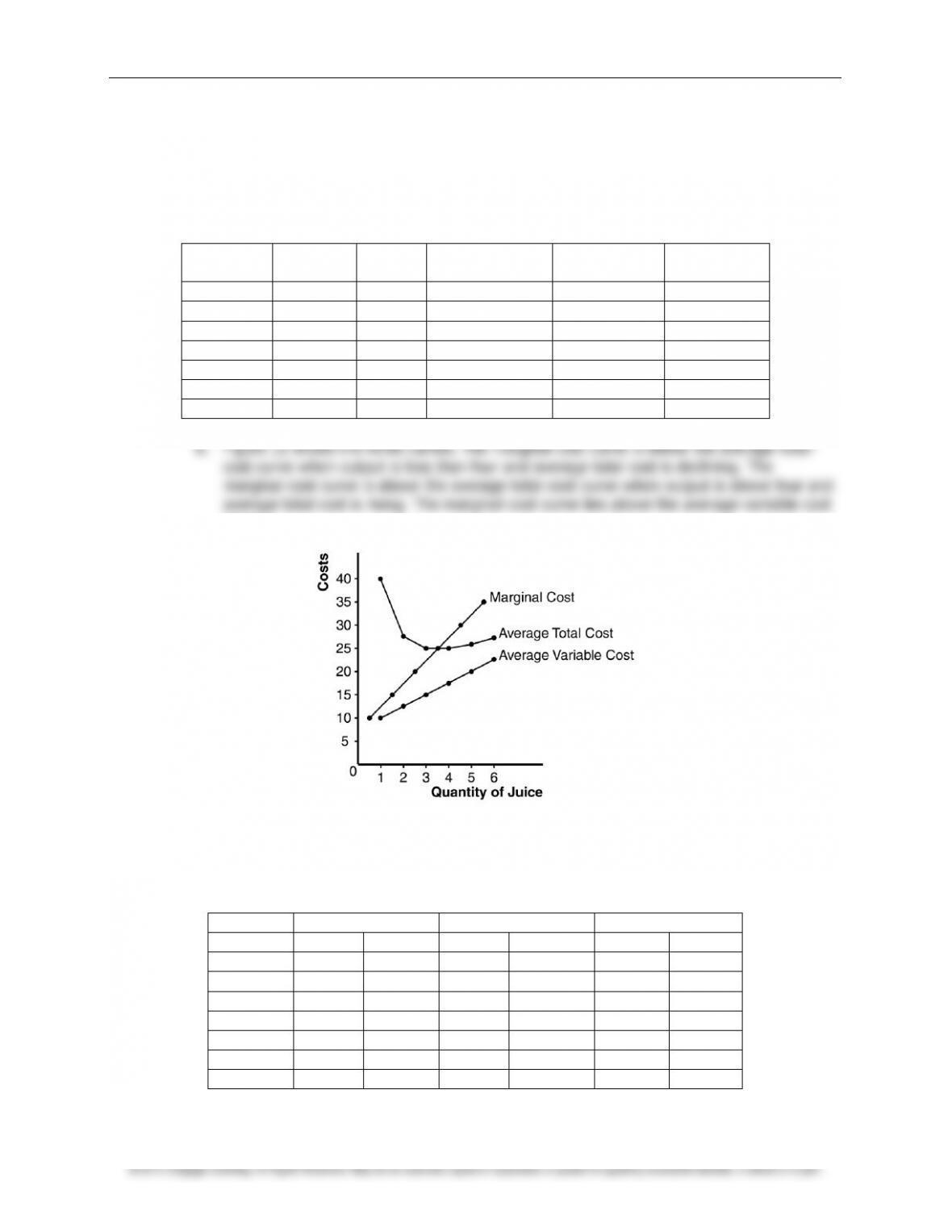
9. a. The following table shows average variable cost (
AVC
), average total cost (
ATC
), and
marginal cost (
MC
) for each quantity.
Quantity
Variable
Cost
Total
Cost
Average
Variable Cost
Average
Total Cost
Marginal
Cost
0
$0.00
$30.00
—
—
—
1
10.00
40.00
$10.00
$40.00
$10.00
2
25.00
55.00
12.50
27.50
15.00
3
45.00
75.00
15.00
25.00
20.00
4
70.00
100.00
17.50
25.00
25.00
5
100.00
130.00
20.00
26.00
30.00
6
135.00
165.00
22.50
27.50
35.00
curve.
Figure 12
10. The following table shows quantity (
Q
), total cost (
TC
), and average total cost (
ATC
) for the
three firms:
Firm A
Firm B
Firm C
Quantity
TC
ATC
TC
ATC
TC
ATC
1
$60.00
$60.00
$11.00
$11.00
$21.00
$21.00
2
70.00
35.00
24.00
12.00
34.00
17.00
3
80.00
26.67
39.00
13.00
49.00
16.33
4
90.00
22.50
56.00
14.00
66.00
16.50
5
100.00
20.00
75.00
15.00
85.00
17.00
6
110.00
18.33
96.00
16.00
106.00
17.67
7
120.00
17.14
119.00
17.00
129.00
18.43

240 ❖ Chapter 13/The Costs of Production
© 2012 Cengage Learning. All Rights Reserved. May not be scanned, copied or duplicated, or posted to a publicly accessible website, in whole or in part.
Firm A has economies of scale because average total cost declines as output increases. Firm
B has diseconomies of scale because average total cost rises as output rises. Firm C has
economies of scale from one to three units of output and diseconomies of scale for levels of
output beyond three units.