221
WHAT’S NEW IN THE SEVENTH EDITION:
There are no major changes to this chapter.
LEARNING OBJECTIVES:
By the end of this chapter, students should understand:
what items are included in a firm’s costs of production.
the link between a firm’s production process and its total costs.
the shape of a typical firm’s cost curves.
the relationship between short-run and long-run costs.
CONTEXT AND PURPOSE:
The purpose of Chapter 13 is to address the costs of production and develop the firm’s cost curves.
These cost curves underlie the firm’s supply curve. In previous chapters, we summarized the firm’s
production decisions by starting with the supply curve. While this is suitable for answering many
part of economics known as
industrial organization
—the study of how firms’ decisions about prices and
quantities depend on the market conditions they face.
KEY POINTS:
THE COSTS OF PRODUCTION
13
222 ❖ Chapter 13/The Costs of Production
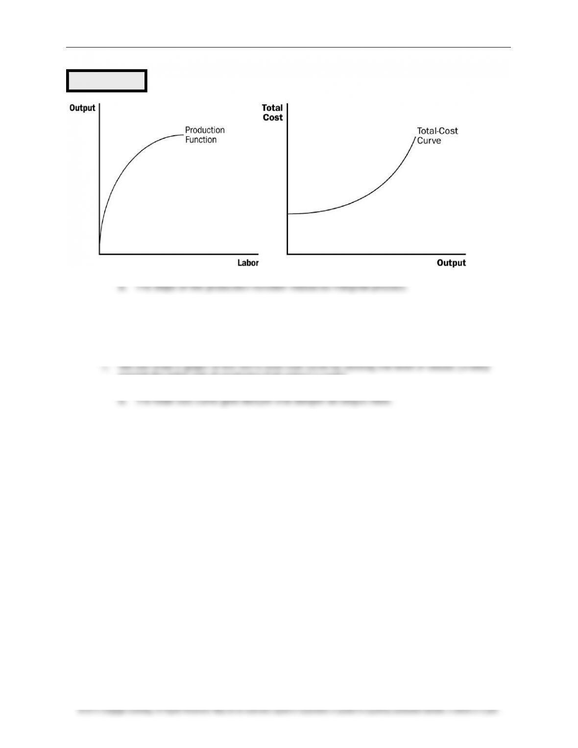
A firm’s costs reflect its production process. A typical firm’s production function gets flatter as the
quantity of an input increases, displaying the property of diminishing marginal product. As a result, a
firm’s total-cost curve gets steeper as the quantity produced rises.
From a firm’s total cost, two related measures of cost are derived. Average total cost is total cost
divided by the quantity of output. Marginal cost is the amount by which total cost rises if output
increases by one unit.
A firm’s costs often depend on the time horizon considered. In particular, many costs are fixed in the
short run but variable in the long run. As a result, when the firm changes its level of production,
average total cost may rise more in the short run than in the long run.
CHAPTER OUTLINE:
I. What Are Costs?
A. Total Revenue, Total Cost, and Profit
1. The goal of a firm is to maximize profit.
This is an extremely important chapter, and it is critical that students have an
understanding of the important principles developed here in order to follow the
material presented in the next several chapters. Do not be surprised at the number
of students who are unfamiliar with such seemingly simple concepts as revenue,
costs, and profits.
Point out to students that it is possible for firm owners to have different goals, but
the one motive that makes the most accurate prediction about how firm managers
behave is the assumption of profit maximization. To help illustrate this sometimes–
controversial assumption, use the analogy of an automobile driver. Ask students to
name an assumption about the goal of most drivers. Most would agree that drivers
behave as if their goal is to get from one place to another in the least amount of
time. This may not explain the behavior of every driver (i.e., “Sunday” drivers), but it
works for most.
Chapter 13/The Costs of Production ❖ 223
2. Definition of total revenue: the amount a firm receives for the sale of its output.
4. Definition of profit: total revenue minus total cost.
B. Costs as Opportunity Costs
2. The costs of producing an item must include all of the opportunity costs of inputs used in
production.
3. Total opportunity costs include both implicit and explicit costs.
firm.
b. Definition of implicit costs: input costs that do not require an outlay of money
by the firm.
d. This is the major way in which accountants and economists differ in analyzing the
performance of a business.
costs.
C. The Cost of Capital as an Opportunity Cost
1. The opportunity cost of financial capital is an important cost to include in any analysis of firm
performance.
2. Example: Caroline uses $300,000 of her savings to start her firm. It was in a savings account
paying 5% interest.
3. Because Caroline could have earned $15,000 per year on this savings, we must include this
opportunity cost. (Note that an accountant would not count this $15,000 as part of the firm’s
costs.)
Total Revenue = Price Quantity
Profit = Total Revenue Total Cost
Students rarely have trouble understanding the concept of explicit costs. However,
they do often have difficulty understanding the nature of implicit costs. Make sure
that they grasp the concept here, because it is important in understanding why firms
continue to operate even if they are earning zero economic profit in the long run.
224 ❖ Chapter 13/The Costs of Production
4. If Caroline had instead borrowed $200,000 from a bank and used $100,000 from her savings,
loan.
D. Economic Profit versus Accounting Profit
1. Figure 1 highlights the differences in the ways in which economists and accountants calculate
profit.
2. Definition of economic profit: total revenue minus total cost, including both explicit
and implicit costs.
b. To understand how industries evolve, we need to examine economic profit.
4. If implicit costs are greater than zero, accounting profit will always exceed economic profit.
II. Production and Costs
A. The Production Function
1. Definition of production function: the relationship between quantity of inputs used
to make a good and the quantity of output of that good.
2. Example: Caroline’s cookie factory. The size of the factory is assumed to be fixed; Caroline
can vary her output (cookies) only by varying the labor used.
Number of
Workers
Output
Marginal Product
of Labor
Cost of
Factory
Cost of
Workers
Total Cost
of Inputs
0
0
—
$30
$0
$30
1
50
50
30
10
40
2
90
40
30
20
50
3
120
30
30
30
60
4
140
20
30
40
70
5
150
10
30
50
80
6
155
5
30
60
90
Figure 1
Table 1
You may want to give students a handout that summarizes the definitions and
provides them an opportunity to practice the calculations in this chapter. (See the
alternative classroom examples.)
It will be beneficial at this point to distinguish between the long run and the short
run. This will help students understand the distinction between fixed inputs and
variable inputs.
Chapter 13/The Costs of Production ❖ 225
unit of input.
a. As the amount of labor used increases, the marginal product of labor falls.
4. We can draw a graph of the firm’s production function by plotting the level of labor (
x
-axis)
against the level of output (
y
-axis).
change in output
Marginal Product of Labor = change in labor
Go through this table, column by column. Make sure that students understand the
calculations involved.
Point out that diminishing marginal returns is a result of fixed inputs and, therefore is
a short-run phenomenon.
ALTERNATIVE CLASSROOM EXAMPLE:
Consider the short-run production of a small firm that makes sweaters. These sweaters are
made using a combination of labor and knitting machines. In the short run, the firm has
signed a lease to rent one machine. Therefore, in the short run, the firm cannot vary the
amount of knitting machines it uses. However, the firm can vary the amount of labor it
employs.
The first two columns in the table below show the production level that the firm can
achieve at various amounts of labor:
Labor (# workers)
Total Output
Marginal Product
0
0
—
1
4
4
2
10
6
3
13
3
4
15
2
5
16
1
226 ❖ Chapter 13/The Costs of Production
b. Diminishing marginal product can be seen from the fact that the slope falls as the
amount of labor used increases.
B. From the Production Function to the Total-Cost Curve
against the total cost of producing that output (
y
-axis).
b. This increase in the slope of the total cost curve is also due to diminishing marginal
product: As Caroline increases the production of cookies, her kitchen becomes
overcrowded, and she needs a lot more labor.
Figure 2
Chapter 13/The Costs of Production ❖ 227
III. The Various Measures of Cost
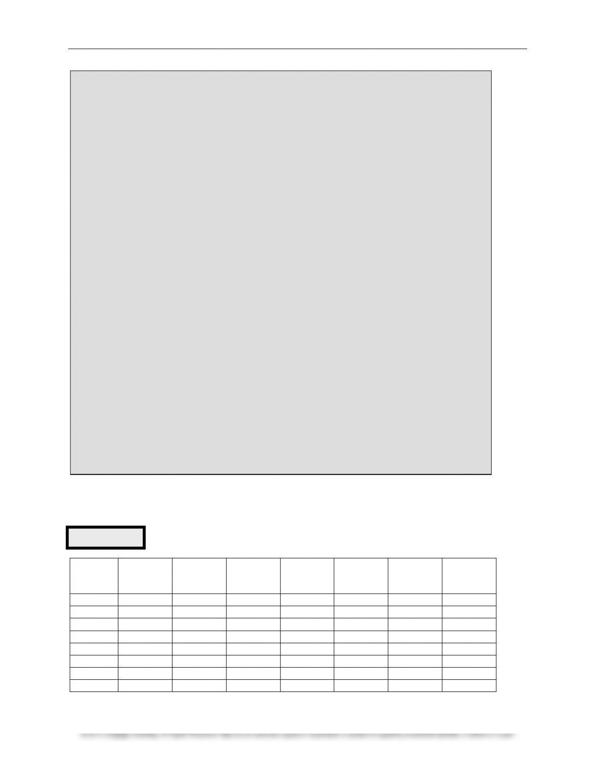
A. Example: Conrad’s Coffee Shop
Output
Total
Cost
Fixed
Cost
Variable
Cost
Average
Fixed
Cost
Average
Variable
Cost
Average
Total
Cost
Marginal
Cost
0
$3.00
$3.00
$0
—
—
—
—
1
3.30
3.00
0.30
$3.00
$0.30
$3.30
$0.30
2
3.80
3.00
0.80
1.50
0.40
1.90
0.50
3
4.50
3.00
1.50
1.00
0.50
1.50
0.70
4
5.40
3.00
2.40
0.75
0.60
1.35
0.90
5
6.50
3.00
3.50
0.60
0.70
1.30
1.10
6
7.80
3.00
4.80
0.50
0.80
1.30
1.30
7
9.30
3.00
6.30
0.43
0.90
1.33
1.50
Activity 1—Growing Rice on a Chalkboard
Type: In-class demonstration
Topics: Diminishing returns and increasing costs
Materials needed: Chalkboard and chalk
Time: 25 minutes
Class limitations: Works in classes with more than 15 students
Purpose
Students often have difficulty understanding why diminishing returns exist in short-run
production. This activity vividly demonstrates how fixed factors constrain the returns to
variable inputs. Then the cause of increasing marginal cost is obvious.
Instructions
Prepare the game by selecting two volunteers and outlining two rectangular areas on the
chalkboard, approximately 2 3 feet. Next to each area, label a column “Labor” and another
“Total Output.” Give each volunteer one piece of chalk and hide any other pieces. The chalk is
a fixed factor of production.
The volunteers are farmers and the outlined areas are their farm fields. They produce rice by
writing the word “RICE” in large letters inside their own field. The letters need to be at least
three inches high. They want to produce as much rice as possible in each 15-second time
period.
The variable input in this example is labor. The game is played repeatedly, adding another
student each period. Eventually five students will be crowded around each “field” trying to
write with a tiny piece of chalk.
The constraints from the fixed factors are physically demonstrated.
Start the game with zeros in both the labor and total output columns; with no labor, no rice is
produced. Then have the two volunteers race to see how much they can produce in 15
seconds. Record their production under “Total Output” with one “Labor.”
Table 2
228 ❖ Chapter 13/The Costs of Production
8
11.00
3.00
8.00
0.38
1.00
1.38
1.70
9
12.90
3.00
9.90
0.33
1.10
1.43
1.90
10
15.00
3.00
12.00
0.30
1.20
1.50
2.10
B. Fixed and Variable Costs
produced.
2. Definition of variable costs: costs that do vary with the quantity of output
produced.
C. Average and Marginal Cost
1. Definition of average total cost: total cost divided by the quantity of output.
3. Definition of average variable cost: variable costs divided by the quantity of output.
of production.
TC VC FC
TC FC VC
change in total cost
change in output
MC
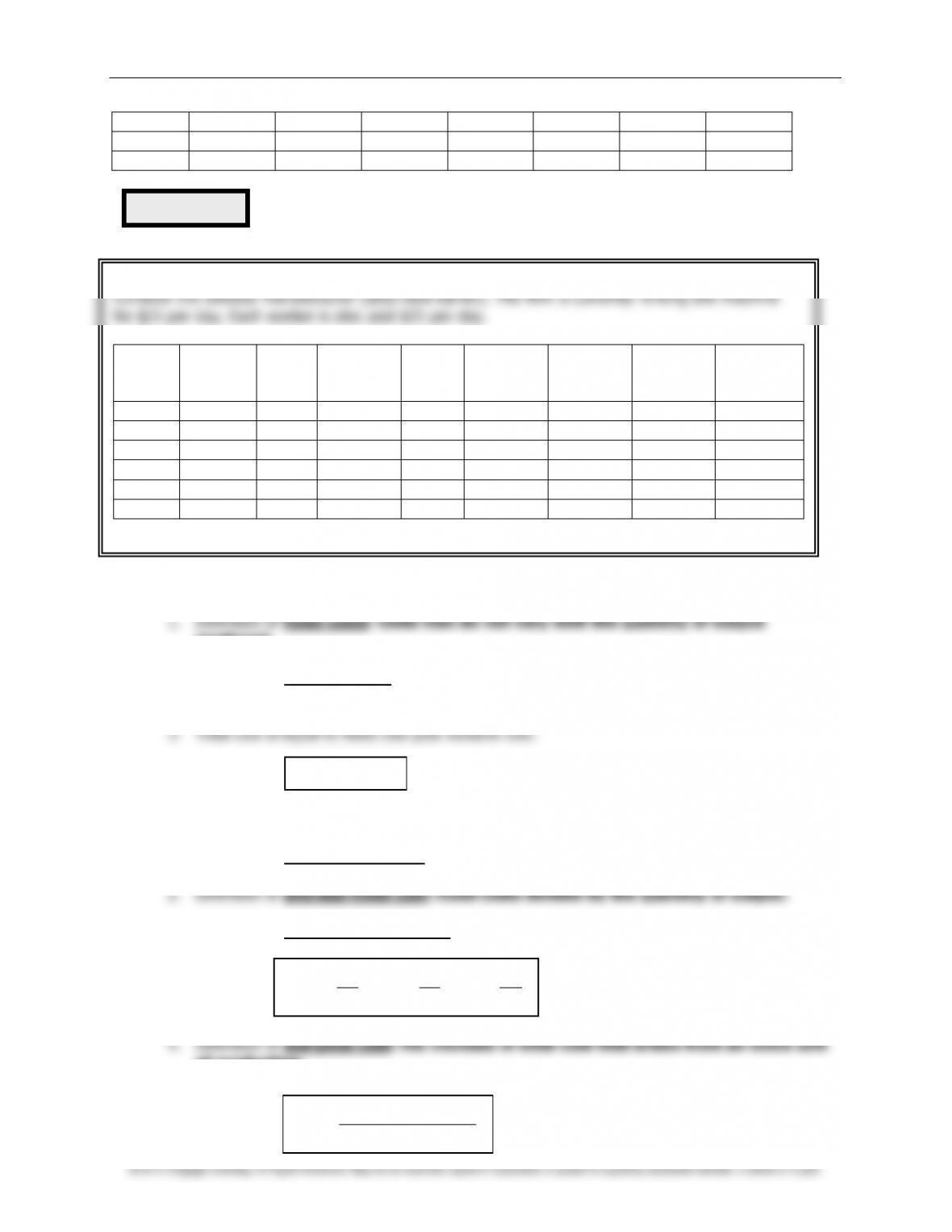
ALTERNATIVE CLASSROOM EXAMPLE:
Consider the sweater manufacturer (described earlier). The firm is currently renting one machine
for $25 per day. Each worker is also paid $25 per day.
Labor
Output
Fixed
Cost
Variable
Cost
Total
Cost
Average
Fixed
Cost
Average
Variable
Cost
Average
Total
Cost
Marginal
Cost
0
0
$25
$0
$25
—-
—-
—-
—-
1
4
25
25
50
$6.25
$6.25
$12.50
$6.25
2
10
25
50
75
2.50
5.00
7.50
4.17
3
13
25
75
100
1.92
5.77
7.69
8.33
4
15
25
100
125
1.67
6.67
8.33
12.50
5
16
25
125
150
1.56
7.81
9.38
25.00
Figure 3
Chapter 13/The Costs of Production ❖ 229
5. Average total cost tells us the cost of a typical unit of output and marginal cost tells us the
cost of an additional unit of output.
D. Cost Curves and Their Shapes
1. Rising Marginal Cost
b. At a low level of output, there are few workers and a lot of idle equipment. But as output
increases, the coffee shop gets crowded and the cost of producing another unit of output
becomes high.
2. U-Shaped Average Total Cost
b.
AFC
declines as output expands and
AVC
typically increases as output expands.
AFC
is
fixed costs get spread over a large number of units, the effect of
AFC
on
ATC
falls and
c. Definition of efficient scale: the quantity of output that minimizes average total
cost.
3. The Relationship between Marginal Cost and Average Total Cost
b. The marginal-cost curve crosses the average-total-cost curve at minimum average total
cost (the efficient scale).
ATC AFC AVC
Figure 4
230 ❖ Chapter 13/The Costs of Production
4. Typical Cost Curves
a. Marginal cost eventually rises with output.
b. The average-total-cost curve is U-shaped.
Activity 2—Average and Marginal Grades
Type: In-class demonstration
Topics: Relationship between marginal and average cost
Materials needed: None
Time: 5 minutes
Class limitations: Works in any size class
Purpose
This quick exercise uses an analogy to illustrate to students that they already know the
relation between marginal values and averages.
Instructions
Tell the class that two twins (Miley and Hannah) are enrolled in Principles of Economics. They
each had a “B” average (GPA = 3.0) before taking the class.
Miley gets a “C” in the course. What happens to her GPA?
Hannah gets an “A” in the class. What happens to her GPA?
Common Answers and Points for Discussion
Students will likely know that Miley will have a lower GPA and Hannah a higher GPA. A
“marginal” grade lower than the average will pull down the average. A “marginal” grade
higher than the average will increase the average.
The same is true of marginal cost and average costs. If marginal cost is less than average
cost, average cost will fall. If marginal cost is higher than average cost, average cost will rise.
Figure 5