
Problem 13-20 Problem 13-23
Spreadsheet Templates
Risk and Capital Budgeting
Spreadsheet Templates by Block, Hirt and Danielsen
Copyright © 2011 McGraw-Hill/Irwin and ANSR Source India Pvt Ltd. (www.ansrsourceindia.com)
MAIN MENU – CHAPTER 13
Foundations of Financial Management

Problem 13-20
Objective: Probability analysis with a normal curve distribution
Student Name:
Course Name:
Student ID:
Course Number:
When returns from a project can be assumed to be normally distributed, such as those shown in Figure 13–6
(represented by a symmetrical, bell-shaped curve), the areas under the curve can be determined from
statistical tables based on standard deviations. For example, 68.26 percent of the distribution will fall
within one standard deviation of the expected value (D ± 1σ). Similarly 95.44 percent will fall within two
standard deviations (D ± 2σ), and so on. An abbreviated table of areas under the normal curve is shown here.
Number of σ’s
from Expected
Value + or – + and –
0.50 0.1915 0.3830
1.00 0.3413 0.6826
1.50 0.4332 0.8664
1.96 0.4750 0.9500
2.00 0.4772 0.9544
Assume project A has an expected value of $30,000 and a standard deviation (σ) of $6,000.
a. What is the probability that the outcome will be between $24,000 and $36,000?
b. What is the probability that the outcome will be between $21,000 and $39,000?
c. What is the probability that the outcome will be at least $18,000?
d. What is the probability that the outcome will be less than $41,760?
e. What is the probability that the outcome will be less than $27,000 or greater than $39,000?
Block, Hirt and Danielsen
Foundations of Financial Management
Problem 13-20
Instructions
Enter formulas to calculate the requirements of this problem
a. What is the probability that the outcome will be between $24,000 and $36,000? 0.6826
b. What is the probability that the outcome will be between $21,000 and $39,000? 0.8664
c. What is the probability that the outcome will be at least $18,000? 0.9772
d. What is the probability that the outcome will be less than $41,760? 0.9750
e. What is the probability that the outcome will be less than $27,000
or greater than $39,000? 0.3753
Solution

Problem 13-23
Objective: Portfolio effect of a merger
Student Name:
Course Name:
Student ID:
Course Number:
Transoceanic Airlines is examining a resort motel chain to add to its operation. Prior to the acquisition, the normal
expected outcomes for the firm are as follows:
Outcomes
($ millions) Probability
Recession $30 0.30
Normal economy 50 0.40
Strong economy 70 0.30
After the acquisition, the expected outcomes for the firm would be:
Outcomes
($ millions) Probability
Recession $10 0.30
Normal economy 50 0.40
Strong economy 100 0.30
a. Compute the expected value, standard deviation, and coefficient of variation prior to the acquisition.
After the acquisition, these values are as follows:
Expected value 53.0 ($ millions)
Standard deviation 34.9 ($ millions)
Coefficient of variation 0.658
b. Comment on whether this acquisition appears desirable to you.
c. Do you think the firm’s stock price is likely to go up as a result of this acquisition?
d. If the firm were interested in reducing its risk exposure, which of the following three industries would you
advise it to consider for an acquisition? Briefly comment on your answer.
(1) Major travel agency
(2) Oil company
(3) Gambling casino
Block, Hirt and Danielsen
Foundations of Financial Management
Problem 13-23
Instructions
Enter formulas to complete the requirements of this problem. To calculate the Standard Deviation in part (a),
use the MS Excel SQRT function.
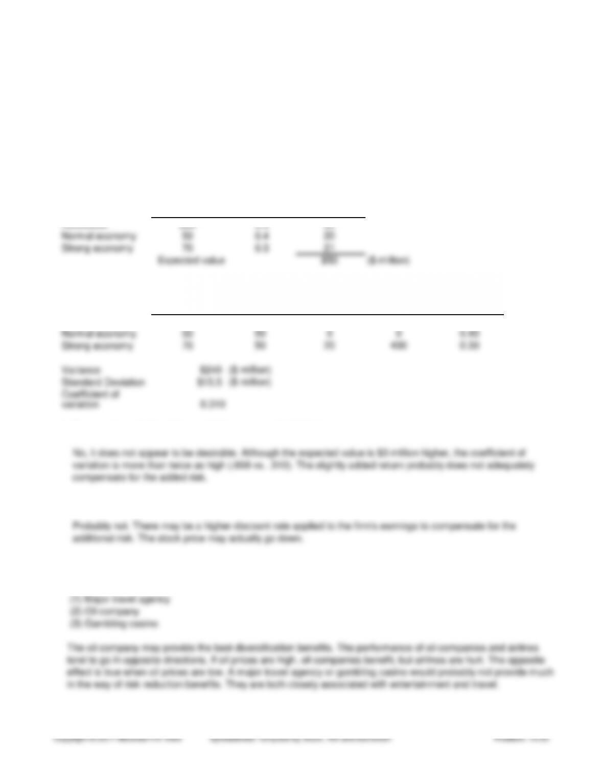
a. Compute the expected value, standard deviation, and coefficient of variation prior to the acquisition.
Outcomes Expected
($ millions) Probability Value
Recession $30 0.3 $9
Normal economy 50 0.4 20
Strong economy 70 0.3 21
Expected value $50 ($ million)
Outcomes Expected Deviations
($ millions) Value Deviations Squared Probability
Strong economy 70 50 20 400 0.30
Variance $240 ($ million)
Standard Deviation $15.5 ($ million)
Coefficient of
variation 0.310
c. Do you think the firm’s stock price is likely to go up as a result of this acquisition?
Probably not. There may be a higher discount rate applied to the firm’s earnings to compensate for the
d. If the firm were interested in reducing its risk exposure, which of the following three industries would you
advise it to consider for an acquisition? Briefly comment on your answer.
(1) Major travel agency
(3) Gambling casino
The oil company may provide the best diversification benefits. The performance of oil companies and airlines
tend to go in opposite directions. If oil prices are high, oil companies benefit, but airlines are hurt. The opposite
effect is true when oil prices are low. A major travel agency or gambling casino would probably not provide much
Solution