18. There are two ways to correctly answer this question so we will work through both. First, we can use
the CAPM. Substituting in the value we are given for each stock, we find:
It is given in the problem that the expected return of Stock Y is 11.1 percent, but according to the
CAPM the expected return of the stock should be 11.04 percent based on its level of risk. This means
the stock return is too high, given its level of risk. Stock Y plots above the SML and is undervalued.
In other words, its price must increase to reduce the expected return to 11.04 percent.
For Stock Z, we find:
The return given for Stock Z is 7.85 percent, but according to the CAPM the expected return of the
We can also answer this question using the reward-to-risk ratio. All assets must have the same
The reward-to-risk ratio for Stock Y is too high, which means the stock plots above the SML, and the
stock is undervalued. Its price must increase until its reward-to-risk ratio is equal to the market
reward-to-risk ratio. For Stock Z, we find:
The reward-to-risk ratio for Stock Z is too low, which means the stock plots below the SML, and the
19. We need to set the reward-to-risk ratios of the two assets equal to each other, which is:
We can cross multiply to get:
Solving for the risk-free rate, we find:
Intermediate
20. a. Again we have a special case where the portfolio is equally weighted, so we can sum the
returns of each asset and divide by the number of assets. The expected return of the portfolio is:
b. We need to find the portfolio weights that result in a portfolio with a beta of .92. We know the
beta of the risk-free asset is zero. We also know the weight of the risk-free asset is one minus
the weight of the stock since the portfolio weights must sum to one, or 100 percent. So:
P = .92 = wS(1.12) + (1 – wS)(0)
And, the weight of the risk-free asset is:
c. We need to find the portfolio weights that result in a portfolio with an expected return of 9
percent. We also know the weight of the risk-free asset is one minus the weight of the stock
since the portfolio weights must sum to one, or 100 percent. So:
E(RP) = .09 = .108wS + .027(1 – wS)
So, the beta of the portfolio will be:
d. Solving for the beta of the portfolio as we did in part a, we find:
P = 2.24 = wS(1.12) + (1 – wS)(0)
The portfolio is invested 200% in the stock and –100% in the risk-free asset. This represents
borrowing at the risk-free rate to buy more of the stock.
21. For a portfolio that is equally invested in large-company stocks and long-term bonds:
For a portfolio that is equally invested in small-company stocks and Treasury bills:
22. We know that the reward-to-risk ratios for all assets must be equal. This can be expressed as:
The numerator of each equation is the risk premium of the asset, so:
We can rearrange this equation to get:
If the reward-to-risk ratios are the same, the ratio of the betas of the assets is equal to the ratio of the
risk premiums of the assets.
23. a. We need to find the return of the portfolio in each state of the economy. To do this, we will
multiply the return of each asset by its portfolio weight and then sum the products to get the
portfolio return in each state of the economy. Doing so, we get:
Boom: RP = .4(.21) + .4(.33) + .2(.55) = .3260, or 32.60%
And the expected return of the portfolio is:
To calculate the standard deviation, we first need to calculate the variance. To find the variance,
we find the squared deviations from the expected return. We then multiply each possible
squared deviation by its probability, then add all of these up. The result is the variance. So, the
variance and standard deviation of the portfolio are:
b. The risk premium is the return of a risky asset minus the risk-free rate. T-bills are often used as
the risk-free rate, so:
c. The approximate expected real return is the expected nominal return minus the inflation rate,
so:
To find the exact real return, we will use the Fisher equation. Doing so, we get:
1 + E(Ri) = (1 + h)[1 + e(ri)]
The approximate real risk-free rate is:
And using the Fisher effect for the exact real risk-free rate, we find:
1 + E(Ri) = (1 + h)[1 + e(ri)]
The approximate real risk premium is the approximate expected real return minus the risk-free
rate, so:
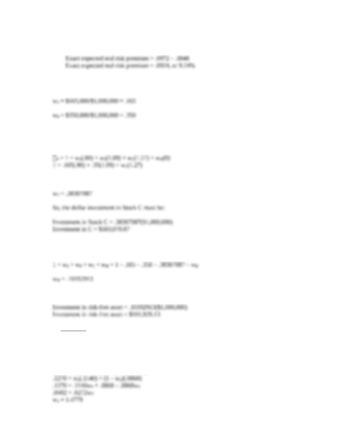
The exact real risk premium is the exact real return minus the exact risk-free rate, so:
24. We know the total portfolio value and the investment in two stocks in the portfolio, so we can find
the weight of these two stocks. The weights of Stock A and Stock B are:
Since the portfolio is as risky as the market, the beta of the portfolio must be equal to one. We also know
the beta of the risk-free asset is zero. We can use the equation for the beta of a portfolio to find the weight
of the third stock. Doing so, we find:
Solving for the weight of Stock C, we find:
So, the dollar investment in Stock C must be:
We also know the total portfolio weight must be one, so the weight of the risk-free asset must be one
minus the asset weights we know, or:
So, the dollar investment in the risk-free asset must be:
Challenge
25. We are given the expected return of the assets in the portfolio. We also know the sum of the weights
of each asset must be equal to one. Using this relationship, we can express the expected return of the
portfolio as:
E(RP) = .1270 = wX(.1140) + wY(.0868)
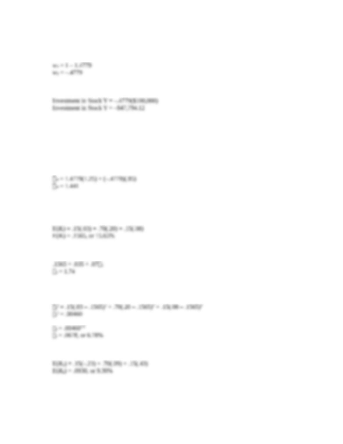
And the weight of Stock Y is:
The amount to invest in Stock Y is:
A negative portfolio weight means that you short sell the stock. If you are not familiar with short
selling, it means you borrow a stock today and sell it. You must then purchase the stock at a later
date to repay the borrowed stock. If you short sell a stock, you make a profit if the stock decreases in
value.
To find the beta of the portfolio, we can multiply the portfolio weight of each asset times its beta and
sum. So, the beta of the portfolio is:
26. The amount of systematic risk is measured by the beta of an asset. Since we know the market risk
premium and the risk-free rate, if we know the expected return of the asset we can use the CAPM to
solve for the beta of the asset. The expected return of Stock I is:
Using the CAPM to find the beta of Stock I, we find:
The total risk of the asset is measured by its standard deviation, so we need to calculate the standard
deviation of Stock I. Beginning with the calculation of the stock’s variance, we find:
Using the same procedure for Stock II, we find the expected return to be:
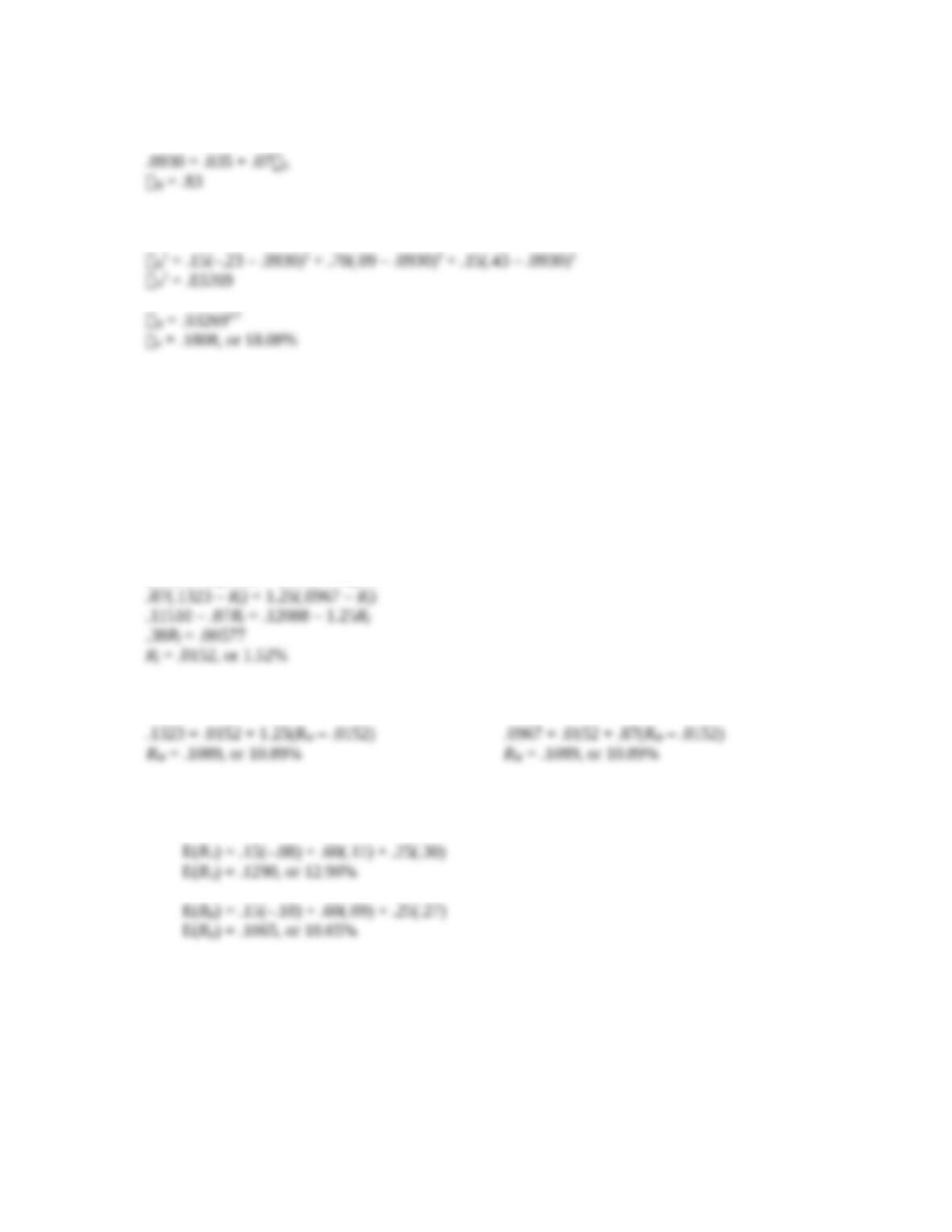
Using the CAPM to find the beta of Stock II, we find:
And the standard deviation of Stock II is:
Although Stock II has more total risk than I, it has much less systematic risk, since its beta is much
smaller than I’s. Thus, I has more systematic risk, and II has more unsystematic and total risk. Since
unsystematic risk can be diversified away, I is actually the “riskier” stock despite the lack of
volatility in its returns. Stock I will have a higher risk premium and a greater expected return.
27. Here we have the expected return and beta for two assets. We can express the returns of the two
assets using CAPM. If the CAPM is true, then the security market line holds as well, which means
all assets have the same risk premium. Setting the risk premiums of the assets equal to each other
and solving for the risk-free rate, we find:
(.1323 – Rf)/1.25 = (.0967 – Rf)/.87
Now using CAPM to find the expected return on the market with both stocks, we find:
28. a. The expected return of an asset is the sum of the probability of each return occurring times the
probability of that return occurring. So, the expected return of each stock is:
b. We can use the expected returns we calculated to find the slope of the SML. We know that the
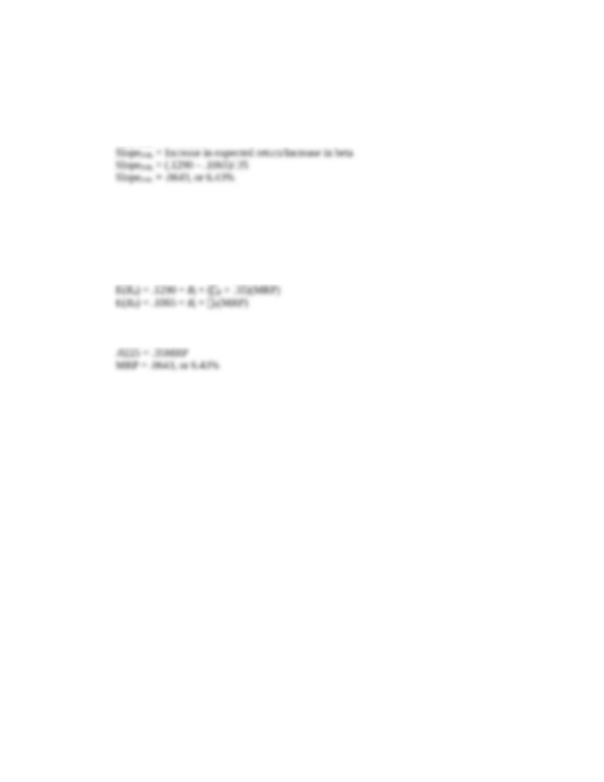
beta of Stock A is .35 greater than the beta of Stock B. Therefore, as beta increases by .35, the
expected return on a security increases by .0225 (= .1290 – .1065). The slope of the SML
equals:
SlopeSML = Rise/Run
Since the market’s beta is 1 and the risk-free rate has a beta of zero, the slope of the SML
equals the expected market risk premium. So, the expected market risk premium must be 6.43
percent.
We could also solve this problem using CAPM. The equations for the expected returns of the
two stocks are:
Subtracting the CAPM equation for Stock B from the CAPM equation for Stock A yields:
which is the same answer as our previous result.