CHAPTER 12
SOME LESSONS FROM CAPITAL
MARKET HISTORY
Answers to Concepts Review and Critical Thinking Questions
3. Not necessarily, because stocks are riskier. Some investors are highly risk averse, and the extra
4. On average, the only return that is earned is the required return—investors buy assets with returns in
7. Ignoring trading costs, on average, such investors merely earn what the market offers; stock
8. Unlike gambling, the stock market is a positive sum game; everybody can win. Also, speculators
9. The EMH only says, within the bounds of increasingly strong assumptions about the information
processing of investors, that assets are fairly priced. An implication of this is that, on average, the
10. a. If the market is not weak form efficient, then this information could be acted on and a profit
CHAPTER 12 – 2
b. Under (2), if the market is not semi-strong form efficient, then this information could be used to
c. Under (3), if the market is not strong form efficient, then this information could be used as a
profitable trading strategy, by noting the buying activity of the insiders as a signal that the stock
Solutions to Questions and Problems
NOTE: All end of chapter problems were solved using a spreadsheet. Many problems require multiple
steps. Due to space and readability constraints, when these intermediate steps are included in this
solutions manual, rounding may appear to have occurred. However, the final answer for each problem is
found without rounding during any step in the problem.
Basic
1. The return of any asset is the increase in price, plus any dividends or cash flows, all divided by the
initial price. The return of this stock is:
2. The dividend yield is the dividend divided by the beginning of the period price, so:
And the capital gains yield is the increase in price divided by the initial price, so:
3. Using the equation for total return, we find:
And the dividend yield and capital gains yield are:
CHAPTER 12 – 3
Here’s a question for you: Can the dividend yield ever be negative? No, that would mean you were
paying the company for the privilege of owning the stock. However, this has happened on bonds.
4. The total dollar return is the increase in price plus the coupon payment, so:
The total percentage return of the bond is:
Notice here that we could have used the total dollar return of $45 in the numerator of this equation.
Using the Fisher equation, the real return was:
5. The nominal return is the stated return, which is 12.00 percent. Using the Fisher equation, the real
return was:
6. Using the Fisher equation, the real returns for long-term government and corporate bonds were:
(1 + R) = (1 + r)(1 + h)
7. The average return is the sum of the returns, divided by the number of returns. The average return for each
stock was:
¯
X=
[
∑
i=1
N
xi
]
/N=
[
.12+. 28+. 09−. 07+. 10
]
5=.1040, or 10 . 40
CHAPTER 12 – 4
¯
Y=
[
∑
i=1
N
yi
]
/N=
[
.25+. 34+.13−.27+.14
]
5=.1180, or 11. 80
Remembering back to “sadistics,” we calculate the variance of each stock as:
σ
X2=
[
∑
i=1
N
(
xi−¯
x
)
2
]
/
(
N−1
)
σX2=1
5−1
{
(
. 12−. 104
)
2+
(
. 28−.104
)
2+
(
. 09−.104
)
2+
(
−.07−. 104
)
2+
(
.10−.104
)
2
}
=. 01543
σY2=1
5−1
{
(
. 25−. 118
)
2+
(
. 34−.118
)
2+
(
. 13−. 118
)
2+
(
−. 27−.118
)
2+
(
. 14−.118
)
2
}
=. 05447
The standard deviation is the square root of the variance, so the standard deviation of each stock is:
8. We will calculate the sum of the returns for each asset and the observed risk premium first. Doing so,
we get:
Year Large Co. Stock Return T-Bill Return Risk Premium
1970 3.94% 6.50% 2.56%
a. The average return for large company stocks over this period was:
b. Using the equation for variance, we find the variance for large company stocks over this period
was:
And the standard deviation for large company stocks over this period was:
CHAPTER 12 – 5
Using the equation for variance, we find the variance for T-bills over this period was:
And the standard deviation for T-bills over this period was:
c. The average observed risk premium over this period was:
The variance of the observed risk premium was:
And the standard deviation of the observed risk premium was:
d. Before the fact, for most assets the risk premium will be positive; investors demand
9. a. To find the average return, we sum all the returns and divide by the number of returns, so:
b. Using the equation to calculate variance, we find:
So, the standard deviation is:
10. a. To calculate the average real return, we can use the average return of the asset and the average
inflation rate in the Fisher equation. Doing so, we find:
CHAPTER 12 – 6
b. The average risk premium is the average return of the asset, minus the average risk-free rate,
so, the average risk premium for this asset would be:
RP=R
–
Rf
RP
11. We can find the average real risk-free rate using the Fisher equation. The average real risk-free rate
was:
(1 + R) = (1 + r)(1 + h)
rf
rf
And to calculate the average real risk premium, we can subtract the average risk-free rate from the
average real return. So, the average real risk premium was:
rp=r
–
rf
rp
12. T–bill rates were highest in the early 1980s. This was during a period of high inflation and is
Intermediate
13. To find the real return, we first need to find the nominal return, which means we need the current
price of the bond. Going back to the chapter on pricing bonds, we find the current price is:
So the nominal return is:
And, using the Fisher equation, we find the real return is:
CHAPTER 12 – 7
14. Here we know the average stock return, and four of the five returns used to compute the average
return. We can work the average return equation backward to find the missing return. The average
return is calculated as:
The missing return has to be 26.5 percent. Now we can use the equation for the variance to find:
And the standard deviation is:
15. The arithmetic average return is the sum of the known returns divided by the number of returns, so:
Using the equation for the geometric return, we find:
Remember, the geometric average return will always be less than the arithmetic average return if the
returns have any variation.
16. To calculate the arithmetic and geometric average returns, we must first calculate the return for each
year. The return for each year is:
R1 = ($70.20 – 63.40 + .85)/$63.40 = .1207, or 12.07%
The arithmetic average return was:
And the geometric average return was:
CHAPTER 12 – 8
17. Looking at the long-term corporate bond return history in Figure 12.10, we see that the mean return
Pr(R< –2.1 or R>14.7) 1/3
But we are only interested in one tail here, that is, returns less than –2.1 percent, so:
Pr(R< –2.1) 1/6
You can use the z-statistic and the cumulative normal distribution table to find the answer as well.
Doing so, we find:
z = (X – µ)/
Looking at the z-table, this gives a probability of 15.87%, or:
The range of returns you would expect to see 95 percent of the time is the mean plus or minus 2
standard deviations, or:
The range of returns you would expect to see 99 percent of the time is the mean plus or minus 3
standard deviations, or:
18. The mean return for small company stocks was 16.6 percent, with a standard deviation of 31.9
percent. Doubling your money is a 100 percent return, so if the return distribution is normal, we can
use the z-statistic. So:
z = (X – µ)/
This corresponds to a probability of .447%, or once every 200 years.
Tripling your money would be:
CHAPTER 12 – 9
19. It is impossible to lose more than 100 percent of your investment. Therefore, return distributions are
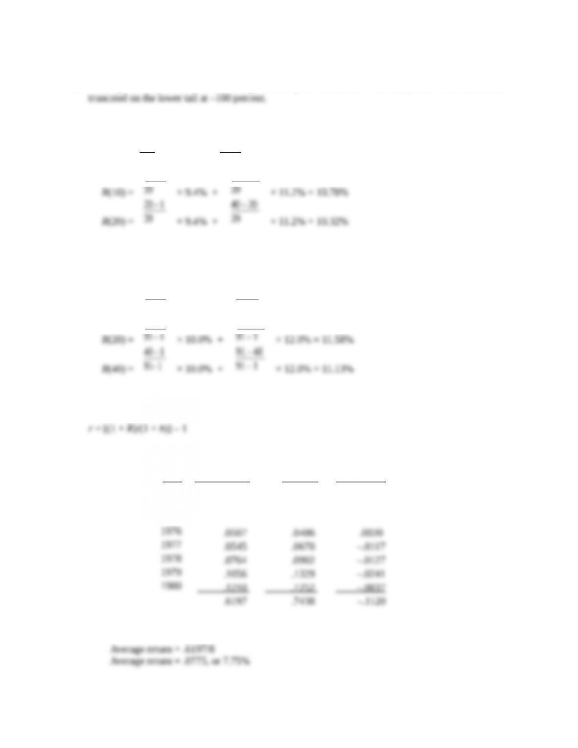
20. To find the best forecast, we apply Blume’s formula as follows:
R(5) =
5 – 1
39
× 9.4% +
40 – 5
39
× 11.2% = 11.02%
20 – 1
39
40 – 20
39
10 – 1
39
40 – 10
39
21. The best forecast for a one year return is the arithmetic average, which is 12.0 percent. The
geometric average, found in Table 12.4 is 10.0 percent. To find the best forecast for other periods, we
apply Blume’s formula as follows:
R(10) =
10 – 1
91 – 1
× 10.0% +
91 – 10
91 – 1
× 12.0% = 11.80%
20 – 1
91 – 1
91 – 20
91 – 1
22. To find the real return we need to use the Fisher equation. Rewriting the Fisher equation to solve for
the real return, we get:
So, the real return each year was:
Year T–Bill Return Inflation Real Return
1973 .0729 .0871 –.0131
1974 .0799 .1234 –.0387
1975 .0587 .0694 –.0100
a. The average return for T-bills over this period was:
CHAPTER 12 – 10
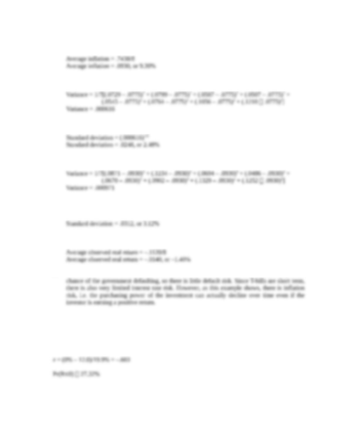
And the average inflation rate was:
b. Using the equation for variance, we find the variance for T-bills over this period was:
And the standard deviation for T-bills was:
The variance of inflation over this period was:
And the standard deviation of inflation was:
Standard deviation = .0009711/2
c. The average observed real return over this period was:
d. The statement that T-bills have no risk refers to the fact that there is only an extremely small
Challenge
23. Using the z-statistic, we find:
z = (X – µ)/
24. For each of the questions asked here, we need to use the z–statistic, which is:
z = (X – µ)/
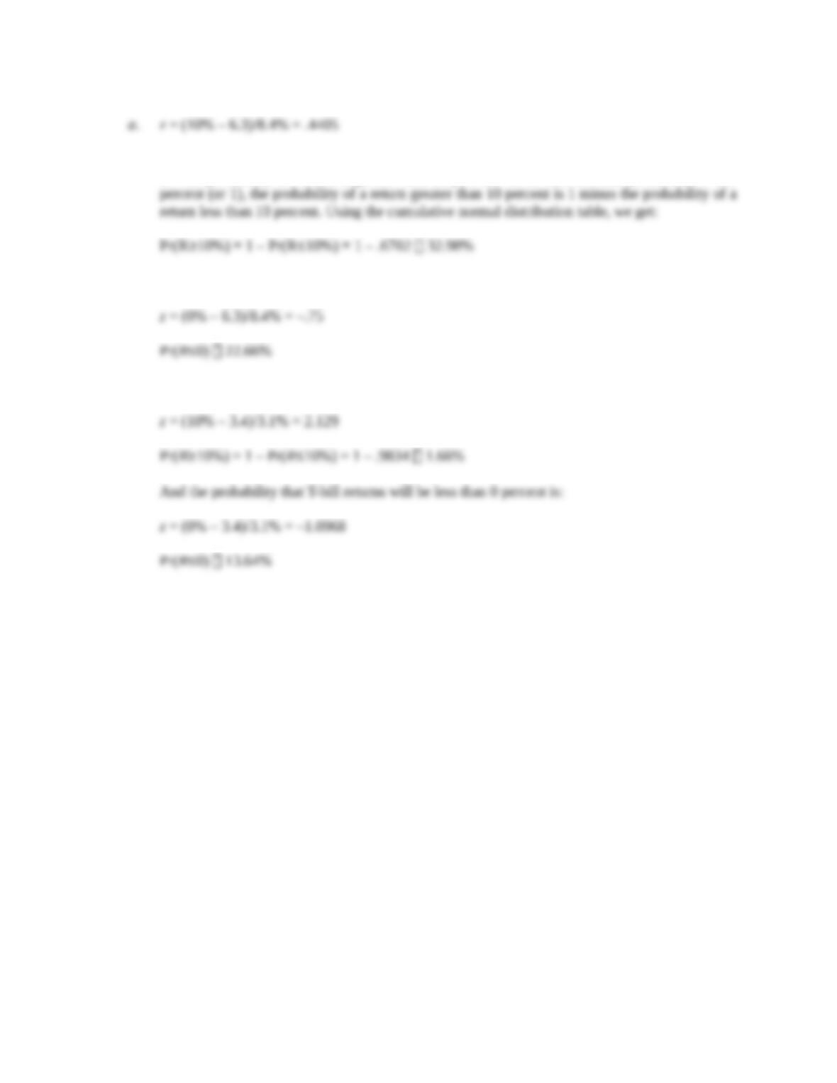
CHAPTER 12 – 11
This z-statistic gives us the probability that the return is less than 10 percent, but we are looking
for the probability the return is greater than 10 percent. Given that the total probability is 100
For a return less than 0 percent:
b. The probability that T-bill returns will be greater than 10 percent is:
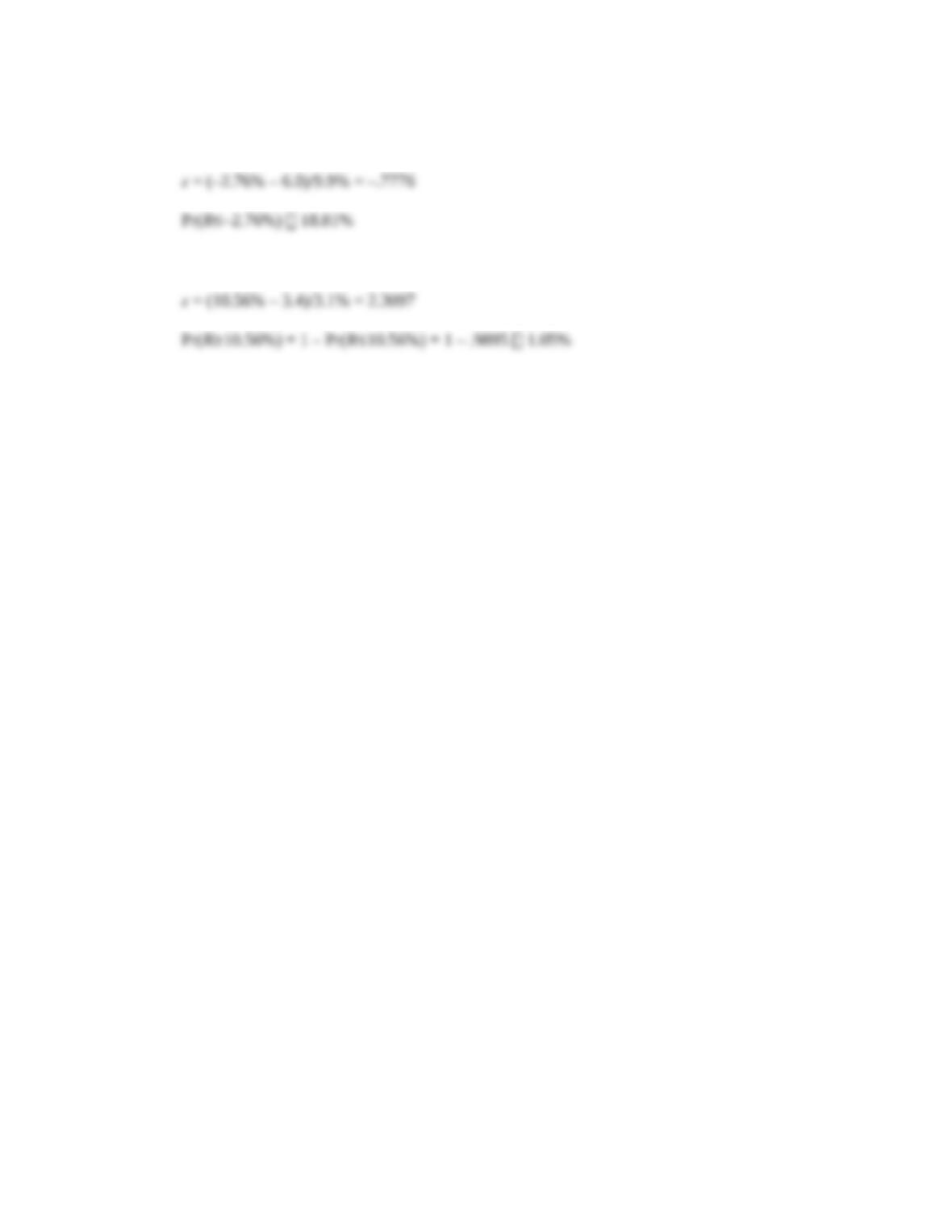
CHAPTER 12 – 12
c. The probability that the return on long-term government bonds will be less than –2.76 percent
is:
And the probability that T-bill returns will be greater than 10.56 percent is:
