CHAPTER 11
PROJECT ANALYSIS AND EVALUATION
Answers to Concepts Review and Critical Thinking Questions
1. Forecasting risk is the risk that a poor decision is made because of errors in projected cash flows.
2. With a sensitivity analysis, one variable is examined over a broad range of values. With a scenario
3. It is true that if average revenue is less than average cost, the firm is losing money. This much of the
5. Fixed costs are relatively high because airlines are relatively capital intensive (and airplanes are
6. From the shareholder perspective, the financial break-even point is the most important. A project can
7. The project will reach the cash break-even first, the accounting break-even next, and finally the
8. Soft capital rationing implies that the firm as a whole isn’t short of capital, but the division or project
does not have the necessary capital. The implication is that the firm is passing up positive NPV
10. While the fact that the worst-case NPV is positive is interesting, it also indicates that there is likely a
CHAPTER 11 – 2
Solutions to Questions and Problems
NOTE: All end of chapter problems were solved using a spreadsheet. Many problems require multiple
steps. Due to space and readability constraints, when these intermediate steps are included in this
solutions manual, rounding may appear to have occurred. However, the final answer for each problem is
found without rounding during any step in the problem.
Basic
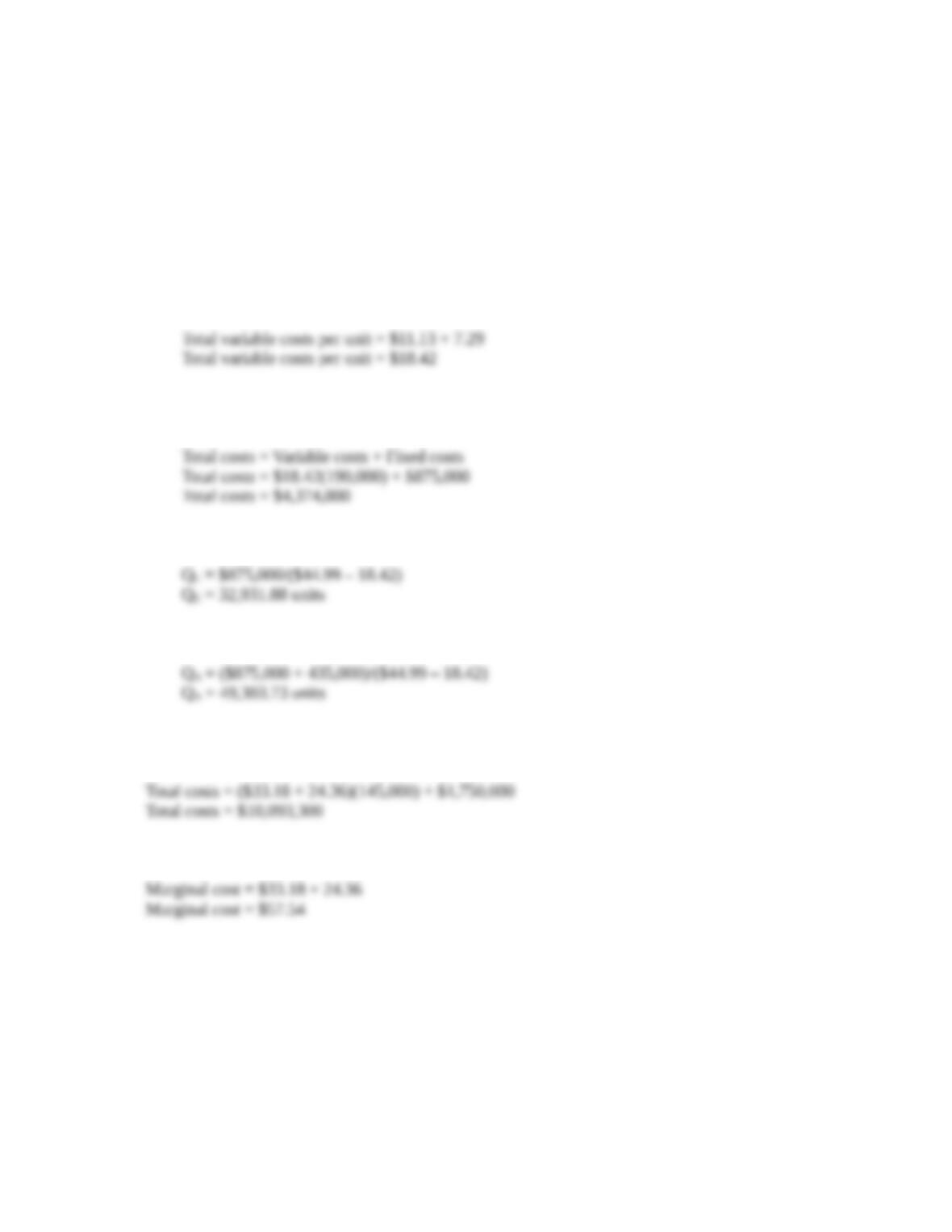
1. a. The total variable cost per unit is the sum of the two variable costs, so:
b. The total costs include all variable costs and fixed costs. We need to make sure we are including
all variable costs for the number of units produced, so:
c. The cash break-even, that is the point where cash flow is zero, is:
And the accounting break-even is:
2. The total costs include all variable costs and fixed costs. We need to make sure we are including all
variable costs for the number of units produced, so:
The marginal cost, or cost of producing one more unit, is the total variable cost per unit, so:
CHAPTER 11 – 3
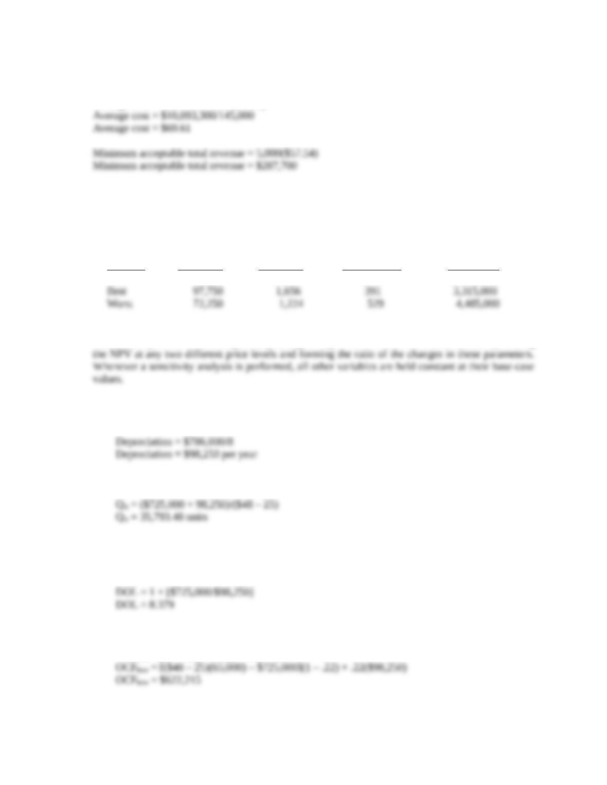
The average cost per unit is the total cost of production, divided by the quantity produced, so:
Average cost = Total cost/Total quantity
Additional units should be produced only if the cost of producing those units can be recovered.
3. The base-case, best-case, and worst-case values are shown below. Remember that in the best-case,
sales and price increase, while costs decrease. In the worst-case, sales and price decrease, and costs
increase.
Unit
Scenario Unit Sales Unit Price Variable Cost Fixed Costs
Base 85,000 $1,440 $460 $3,900,000
4. An estimate for the impact of changes in price on the profitability of the project can be found from
the sensitivity of NPV with respect to price: NPV/P. This measure can be calculated by finding
5. a. To calculate the accounting break-even, we first need to find the depreciation for each year. The
depreciation is:
And the accounting break-even is:
To calculate the accounting break-even, we must realize at this point (and only this point), the
OCF is equal to depreciation. So, the DOL at the accounting break-even is:
DOL = 1 + FC/OCF = 1 + FC/D
b. We will use the tax shield approach to calculate the OCF. The OCF is:
OCFbase = [(P – v)Q – FC](1 – TC) + TCD
CHAPTER 11 – 4
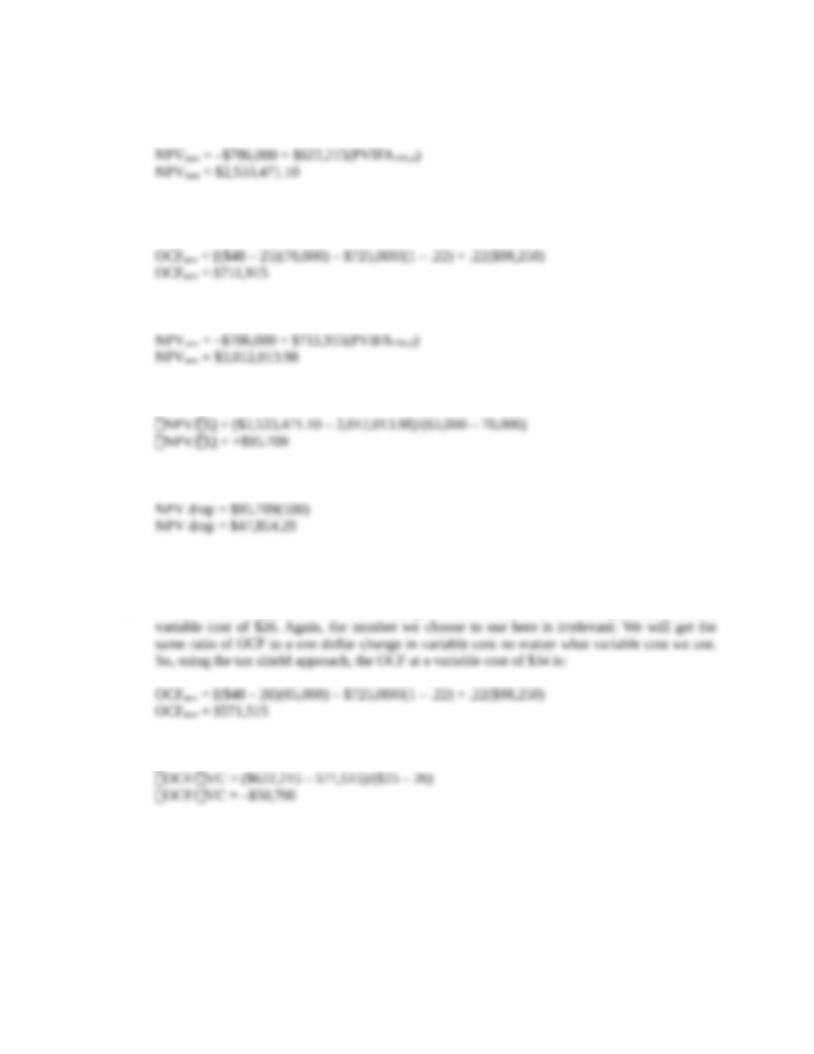
Now we can calculate the NPV using our base-case projections. There is no salvage value or
NWC, so the NPV is:
To calculate the sensitivity of the NPV to changes in the quantity sold, we will calculate the
NPV at a different quantity. We will use sales of 70,000 units. The NPV at this sales level is:
And the NPV is:
So, the change in NPV for every unit change in sales is:
If sales were to drop by 500 units, then NPV would drop by:
You may wonder why we chose 70,000 units. Because it doesn’t matter! Whatever new
quantity we use, when we calculate the change in NPV per unit sold, the ratio will be the same.
c. To find out how sensitive OCF is to a change in variable costs, we will compute the OCF at a
So, the change in OCF for a $1 change in variable costs is:
If variable costs decrease by $1 then OCF would increase by $50,700.
CHAPTER 11 – 5
6. We will use the tax shield approach to calculate the OCF for the best- and worst-case scenarios. For
the best-case scenario, the price and quantity increase by 10 percent, so we will multiply the base-
case numbers by 1.1, a 10 percent increase. The variable and fixed costs both decrease by 10 percent,
so we will multiply the base-case numbers by .9, a 10 percent decrease. Doing so, we get:
The best-case NPV is:
For the worst-case scenario, the price and quantity decrease by 10 percent, so we will multiply the
base-case numbers by .9, a 10 percent decrease. The variable and fixed costs both increase by 10
percent, so we will multiply the base-case numbers by 1.1, a 10 percent increase. Doing so, we get:
The worst-case NPV is:
7. The cash break-even equation is:
QC = FC/(P – v)
And the accounting break-even equation is:
QA = (FC + D)/(P – v)
Using these equations, we find the following cash and accounting break-even points:
a. QC = $8,100,000/($2,980 – 2,135) QA = ($8,100,000 + 3,100,000)/($2,980 – 2,135)
b. QC = $185,000/($46 – 41) QA = ($185,000 + 183,000)/($46 – 41)
c. QC = $2,770/($9 – 3) QA = ($2,770 + 1,050)/($9 – 3)
CHAPTER 11 – 6
8. We can use the accounting break-even equation:
QA = (FC + D)/(P – v)
to solve for the unknown variable in each case. Doing so, we find:
9. The accounting break-even for the project is:
And the cash break-even is:
At the financial break-even, the project will have a zero NPV. Since this is true, the initial cost of the
Using this OCF, we can find the financial break-even is:
And the DOL of the project is:
10. In order to calculate the financial break-even, we need the OCF of the project. We can use the cash
and accounting break-even points to find the OCF. First, we will use the cash break-even to find the
price of the product as follows:
QC = FC/(P – v)
CHAPTER 11 – 7
Now that we know the product price, we can use the accounting break-even equation to find the
depreciation. Doing so, we find the annual depreciation must be:
QA = (FC + D)/(P – v)
We now know the annual depreciation amount. Assuming straight-line depreciation is used, the
initial investment in equipment must be five times the annual depreciation, or:
The PV of the OCF must be equal to this value at the financial break-even since the NPV is zero, so:
We can now use this OCF in the financial break-even equation to find the financial break-even sales
quantity:
11. We know that the DOL is the percentage change in OCF divided by the percentage change in
DOL = %OCF/%Q
Solving for the percentage change in OCF, we get:
%OCF = (DOL)(%Q)
The new level of operating leverage is lower since FC/OCF is smaller.
12. Using the DOL equation, we find:
DOL = 1 + FC/OCF
The percentage change in quantity sold at 43,000 units is:
CHAPTER 11 – 8
So, using the same equation as in the previous problem, we find:
So, the new OCF level will be:
And the new DOL will be:
13. The DOL of the project is:
If the quantity sold changes to 11,100 units, the percentage change in quantity sold is:
So, the OCF at 11,100 units sold is:
%OCF = DOL(%Q)
This makes the new OCF:
And the DOL at 11,100 units is:
CHAPTER 26 – 9