978-1260153132 Chapter 5 Part 9

Solutions Manual, Chapter 5 81

Case 5-32 (continued)

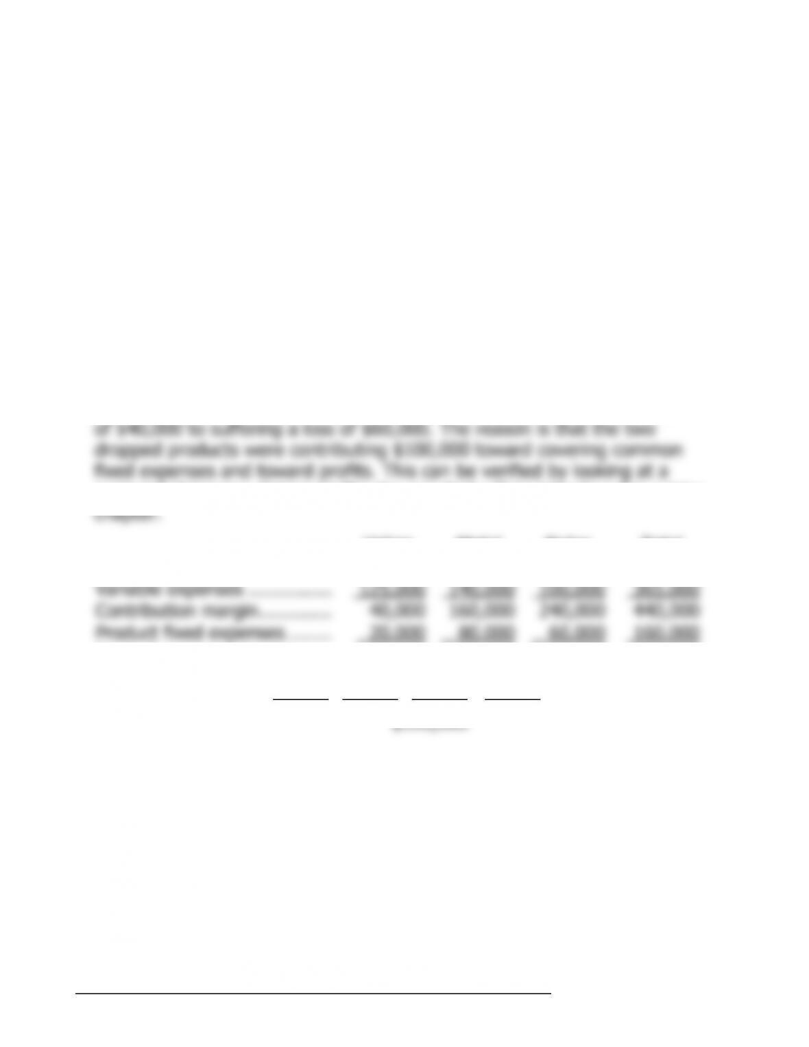
If the managers drop the Velcro and Metal products, the company would

face a loss of $60,000 computed as follows:

Velcro Metal Nylon Total

Sales ……………………… dropped dropped $340,000 $340,000

V

g

* By dropping the two products, the company reduces its fixed expenses

By dropping the two products, the company would go from making a profit

of $40,000 to suffering a loss of $60,000. The reason is that the two

Velcro Metal Nylon Total

Sales ……………………………. $165,000 $300,000 $340,000 $805,000

V

ariable expenses …………… 125,000 140,000 100,000 365,000

Contribution mar

g

in …………. 40,000 160,000 240,000 440,000

82 Managerial Accounting, 16th Edition

Case 5-33 (75 minutes)

Before proceeding with the solution, it is helpful first to restructure the data into contribution format for

each of the three alternatives. (The data in the statements below are in thousands.)

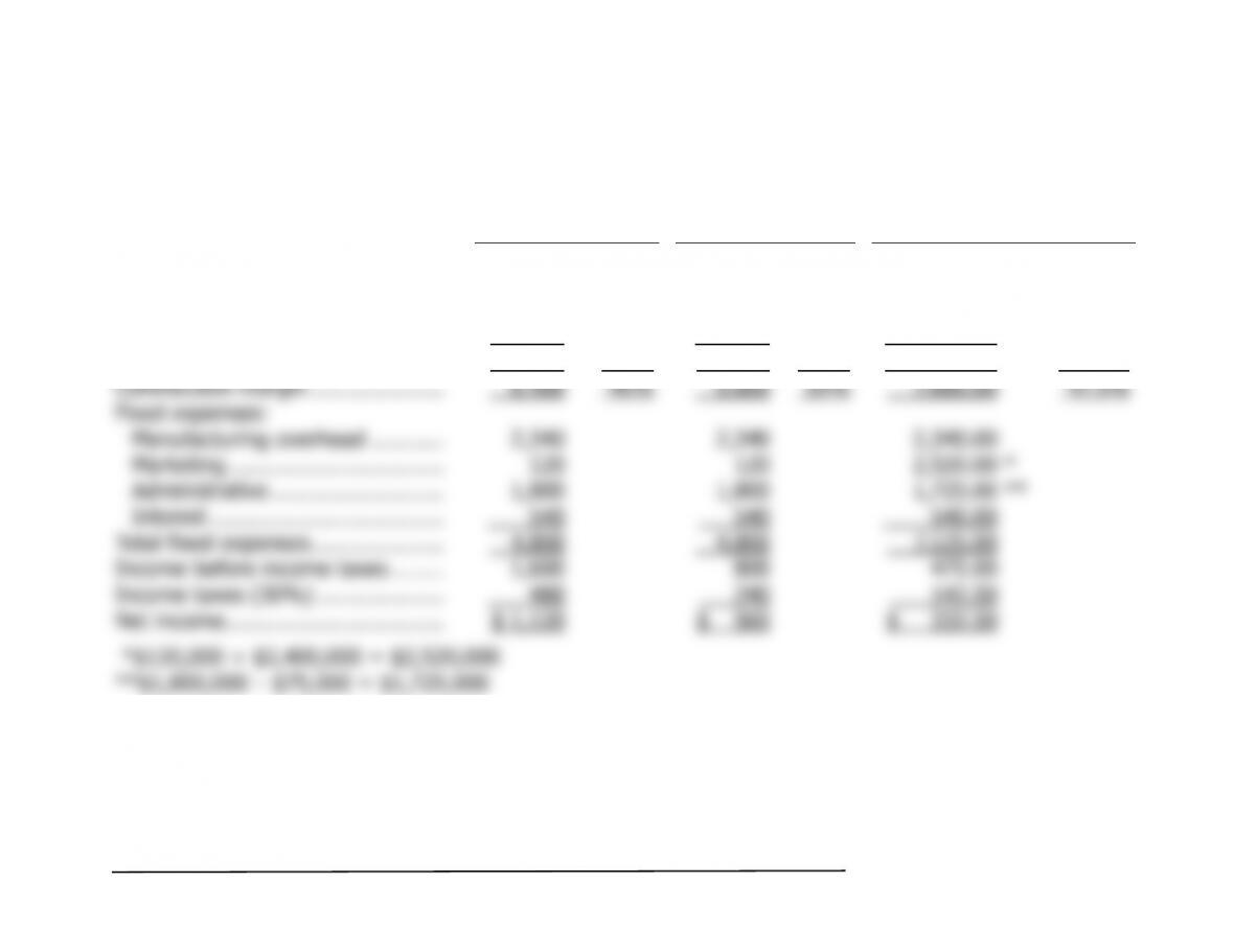
15% Commission 20% Commission Own Sales Force

Sales …………………………………… $16,000 100% $16,000 100% $16,000.00 100.0%

V

ariable expenses:

Manufacturin

g

…………………….. 7,200 7,200 7,200.00

Commissions (15%, 20% 7.5%) 2,400 3,200 1,200.00

T

otal variable expenses …………… 9,600 60% 10,400 65% 8,400.00 52.5%

A

T

–

g

Solutions Manual, Chapter 5 83

Case 5-33 (continued)

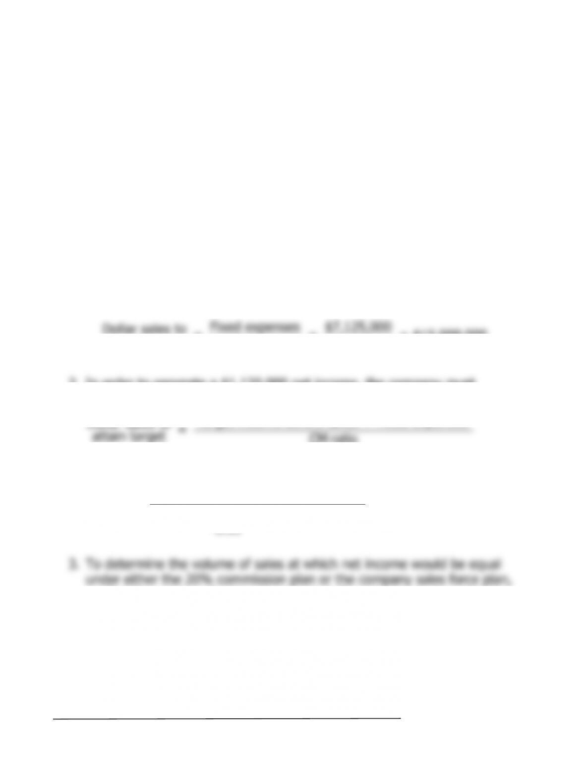
1. When the income before taxes is zero, income taxes will also be zero

and net income will be zero. Therefore, the break-even calculations can

be based on the income before taxes.

a. Break-even point in dollar sales if the commission remains 15%:

b. Break-even point in dollar sales if the commission increases to 20%:

c. Break-even point in dollar sales if the company employs its own sales

force:

2. In order to generate a $1,120,000 net income, the company must

generate $1,600,000 in income before taxes. Therefore,

T

ar

g

et income before taxes + Fixed expenses

Dollar sales to =

attain target CM ratio

3. To determine the volume of sales at which net income would be equal

under either the 20% commission plan or the company sales force plan,

84 Managerial Accounting, 16th Edition

Case 5-33 (continued)

X =

T

otal sales revenue

0.65X + $4,800,000 = 0.525X + $7,125,000

Thus, at a sales level of $18,600,000 either plan would yield the same

income before taxes and net income. Below this sales level, the

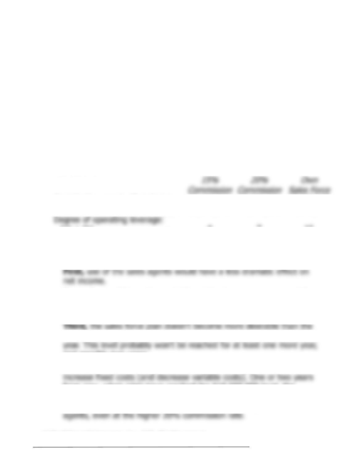
4. a., b., and c.

15%

Commission

20%

Commission

Own

Sales Force

Contribution mar

g

in (Part 1) (a) …. $6,400,000 $5,600,000 $7,600,000

5. We would continue to use the sales agents for at least one more year,

and possibly for two more years. The reasons are as follows:

First, use of the sales agents would have a less dramatic effect on

Second, use of the sales agents for at least one more year would

Third, the sales force plan doesn’t become more desirable than the

use of sales agents until the company reaches sales of $18,600,000 a

Fourth, the sales force plan will be highly leveraged since it will

increase fixed costs (and decrease variable costs). One or two years

from now, when sales have reached the $18,600,000 level, the

Solutions Manual, Appendix 5A 85

Appendix 5A

Analyzing Mixed Costs

Exercise 5A-1 (20 minutes)

1.

Occupancy-

Days

Electrical

Costs

Hi

g

h activity level (Au

g

ust) .. 2,406 $5,148

Low activity level (October) . 124 1,588

Chan

g

e ………………………… 2,282 $3,560

2. Electrical costs may reflect seasonal factors other than just the variation

in occupancy days. For example, common areas such as the reception

Additionally, fixed costs will be affected by the number of days in a

month. In other words, costs like the costs of lighting common areas are

Other, less systematic, factors may also affect electrical costs such

86 Managerial Accounting, 16th Edition

Exercise 5A-2 (20 minutes)

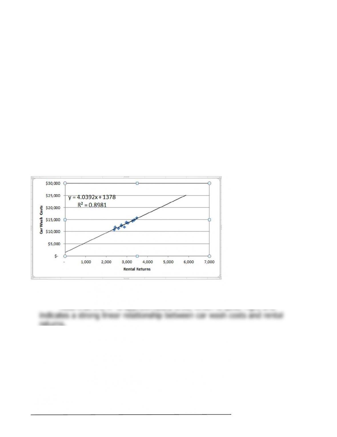
1. and 2.

The scattergraph plot and least-squares regression estimates of fixed and

variable costs using Microsoft Excel are shown below:

The intercept provides the estimate of the fixed cost element, $1,378 per

month, and the slope provides the estimate of the variable cost element,

where X is the number of rental returns.

Note that the R

2

is approximately 0.90, which is quite high, and

Solutions Manual, Appendix 5A 87

Exercise 5A-3 (20 minutes)

1.

Kilometers

Driven

Total Annual

Cost*

Hi

g

h level of activity ……………………. 105,000 $11,970

Variable cost per kilometer:

Change in cost $2,590

= =$0.074 per kilometer

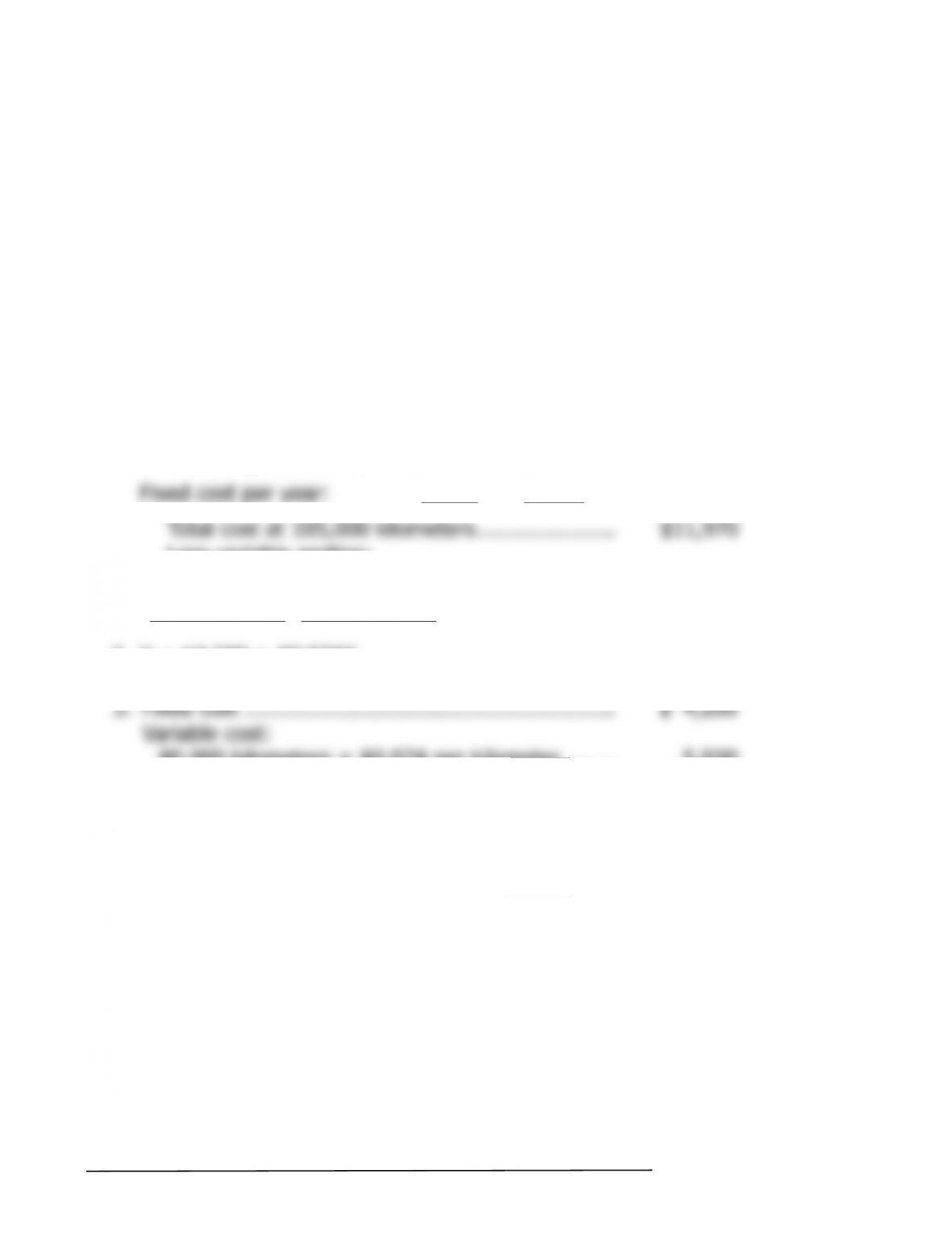
Fixed cost per year:

T

otal cost at 105,000 kilometers………………… $11,970

2. Y = $4,200 + $0.074X

3. Fixed cost ………………………………………….……. $ 4,200

V

T

88 Managerial Accounting, 16th Edition

Exercise 5A-4 (45 minutes)

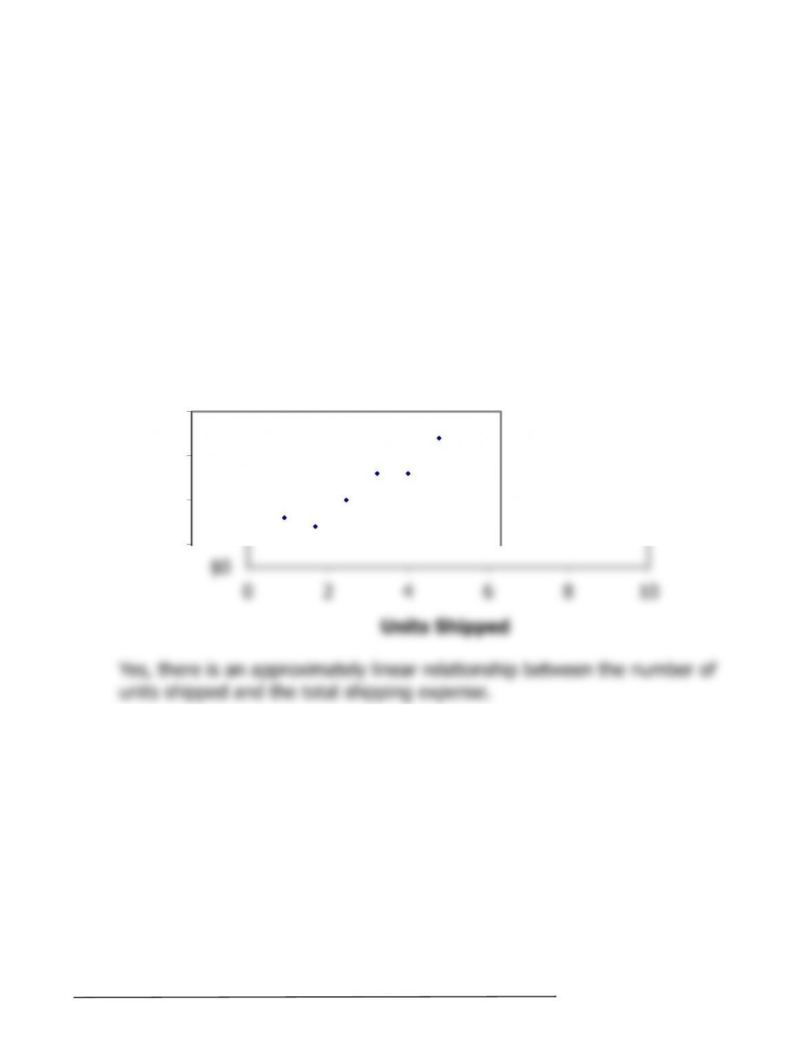
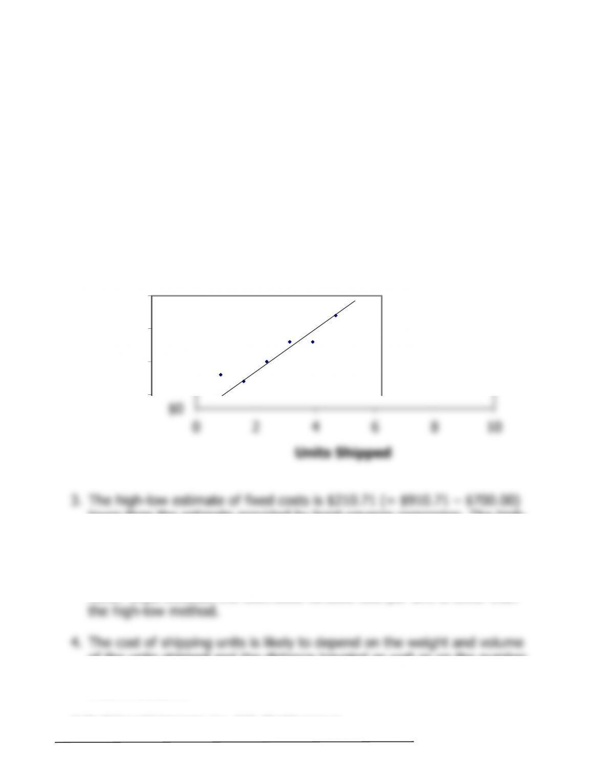
1. The scattergraph appears below:

Yes, there is an approximately linear relationship between the number of

$2,000

$2,500

$3,000

Units Shipped

Solutions Manual, Appendix 5A 89

Exercise 5A-4 (continued)

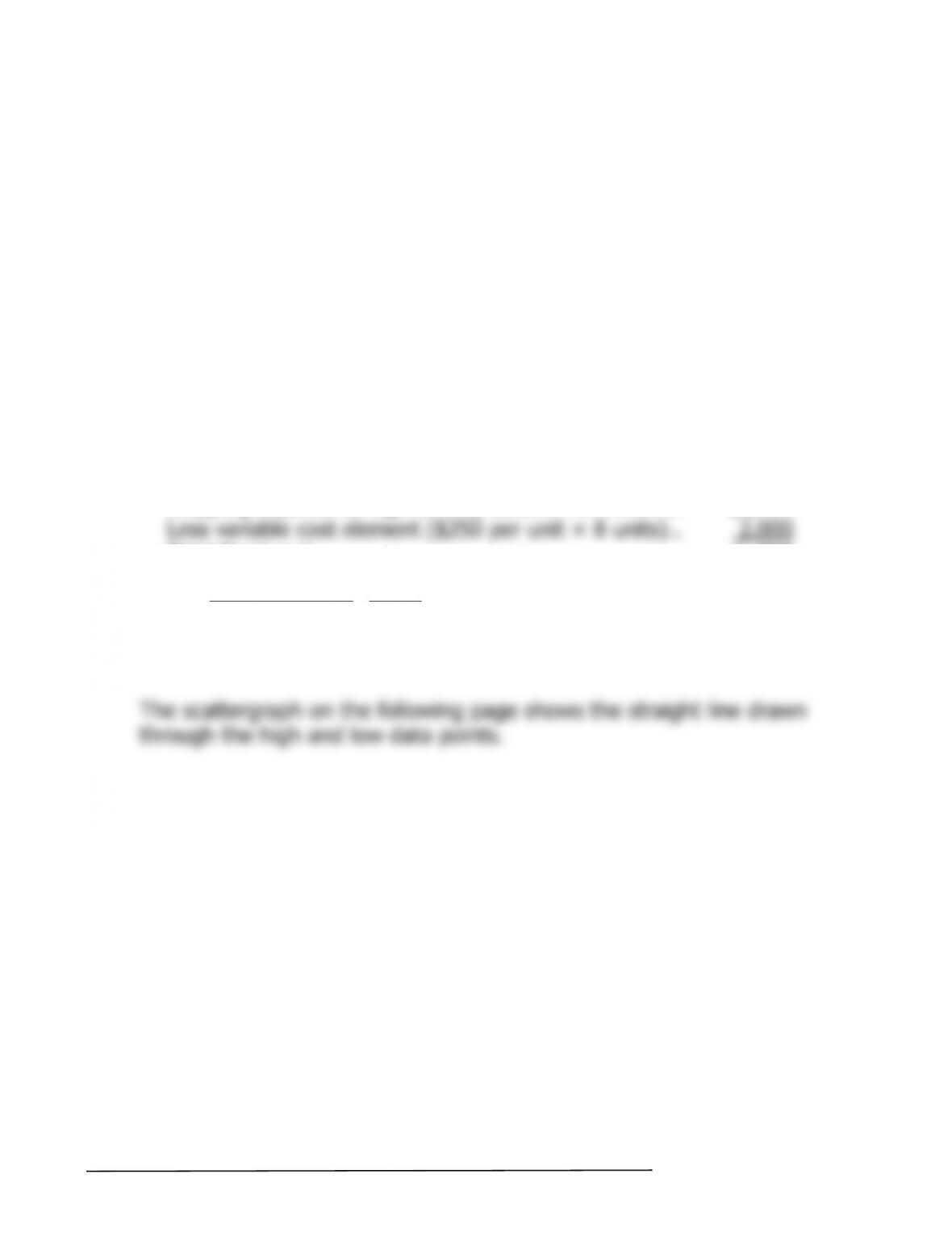
2. The high-low estimates and cost formula are computed as follows:

Units Shipped Shipping Expense

Hi

g

h activity level (June) ….. 8 $2,700

Variable cost element:

Change in expense $1,500

= =$250 per unit.

Change in activity 6 units

Fixed cost element:

Shippin

g

expense at hi

g

h activity level…………………. $2,700

where X is the number of units shipped.

90 Managerial Accounting, 16th Edition

Exercise 5A-4 (continued)

3. The high-low estimate of fixed costs is $210.71 (= $910.71 – $700.00)

lower than the estimate provided by least-squares regression. The high-

low estimate of the variable cost per unit is $32.14 (= $250.00 –

4. The cost of shipping units is likely to depend on the weight and volume

of the units shipped and the distance traveled as well as on the number

$2,000

$2,500

$3,000

Units Shipped