© The McGraw-Hill Companies, Inc., 2018. All rights reserved.
Solutions Manual, Chapter 5 11
The Foundational 15
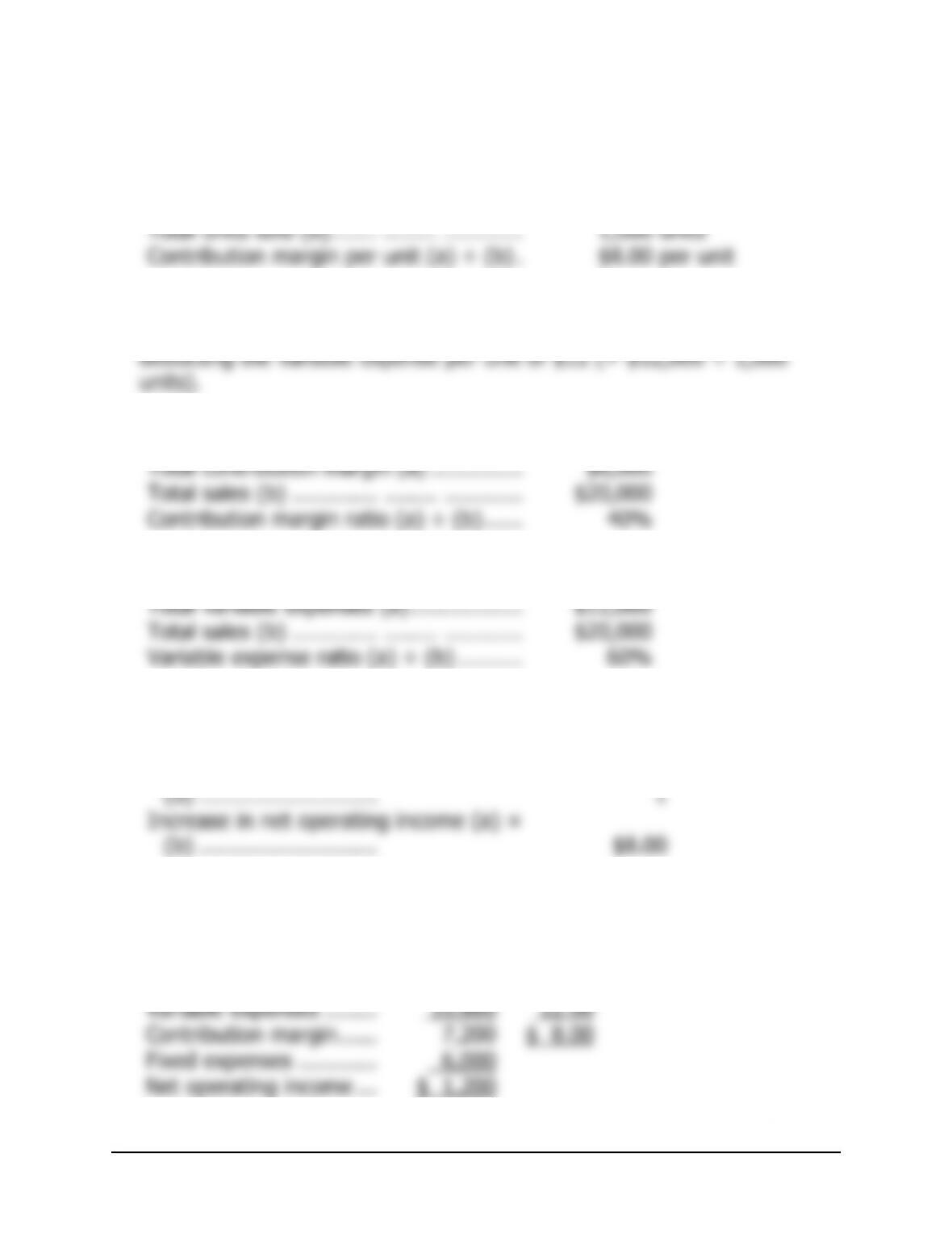
1. The contribution margin per unit is calculated as follows:
T
otal contribution mar
g
in (a) ………….. $8,000
T
g
The contribution margin per unit ($8) can also be derived by calculating
the selling price per unit of $20 (= $20,000 ÷ 1,000 units) and
2. The contribution margin ratio is calculated as follows:
T
g
T
g
3. The variable expense ratio is calculated as follows:
T
T
V
4. The increase in net operating is calculated as follows:
Contribution mar
g
in per unit (a)……..………. $8.00 per unit
Increase in unit sales
unit
5. If sales decline to 900 units, the net operating would be computed as
follows:
T
ota
l
Per Uni
t
Sales (900 units) ………. $18,000 $20.00
V
g
© The McGraw-Hill Companies, Inc., 2018. All rights reserved.
12 Managerial Accounting, 16th Edition
The Foundational 15 (continued)
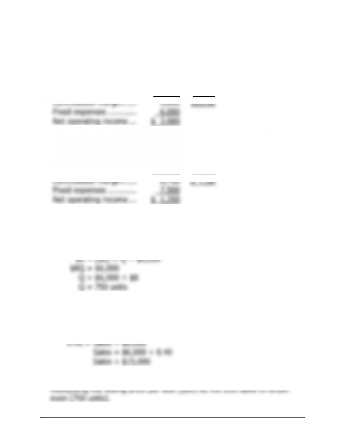
6. The new net operating income would be computed as follows:
T
ota
l
Per Uni
t
Sales (900 units) ………. $19,800 $22.00
V
ariable expenses …….. 10,800 12.00
7. The new net operating income would be computed as follows:
T
ota
l
Per Uni
t
Sales (1,250 units) ……. $25,000 $20.00
V
ariable expenses …….. 16,250 13.00
8. The equation method yields the break-even point in unit sales, Q, as
follows:
Profit = Unit CM × Q − Fixed expenses
$0 = ($20 − $12) × Q − $6,000
9. The equation method yields the dollar sales to break-even as follows:
Profit = CM ratio × Sales − Fixed expenses
$0 = 0.40 × Sales − $6,000
The dollar sales to break-even ($15,000) can also be computed by
© The McGraw-Hill Companies, Inc., 2018. All rights reserved.
Solutions Manual, Chapter 5 13
The Foundational 15 (continued)
10. The equation method yields the target profit as follows:
Profit = Unit CM × Q − Fixed expenses
$5,000 = ($20 − $12) × Q − $6,000
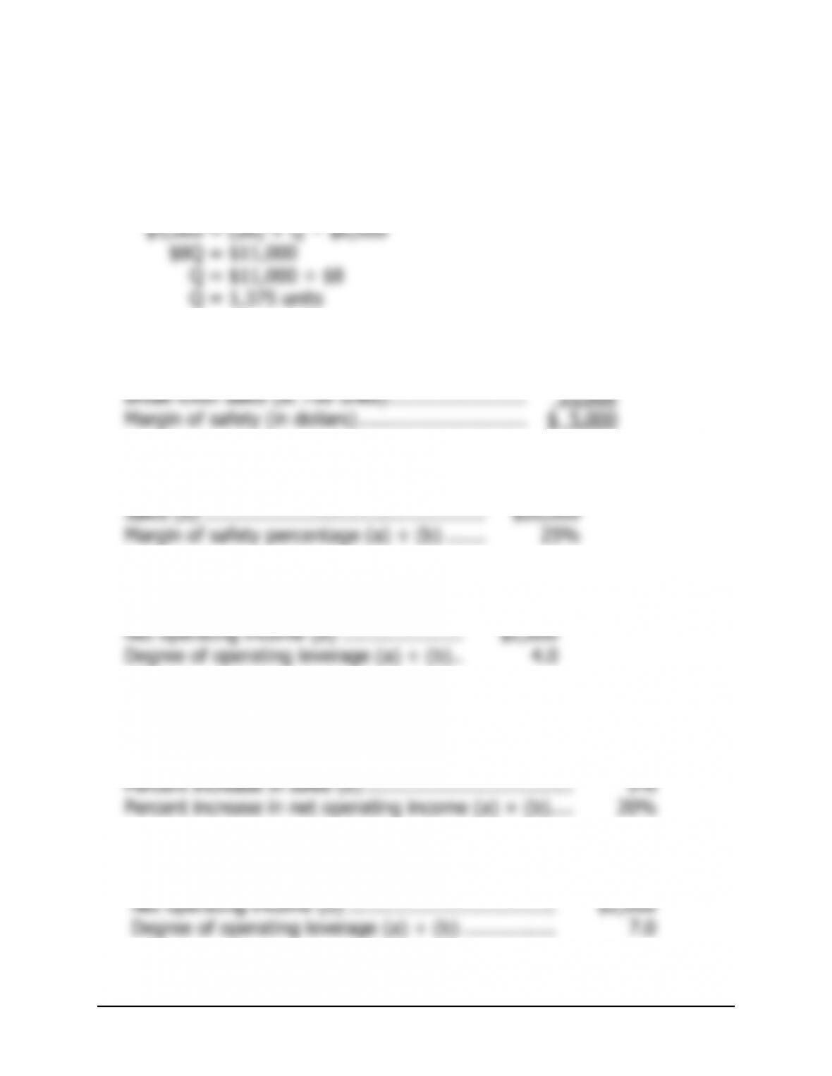
11. The margin of safety in dollars is calculated as follows:
Sales ………………………………………………..….. $20,000
g
The margin of safety as a percentage of sales is calculated as follows:
Mar
g
in of safety (in dollars) (a)…………….. $5,000
g
12. The degree of operating leverage is calculated as follows:
Contribution mar
g
in (a) . …………………. $8,000
g
g
13. A 5% increase in sales should result in a 20% increase in net
operating income, computed as follows:
De
g
ree of operatin
g
levera
g
e (a) ……………………….. 4.0
14. The degree of operating leverage is calculated as follows:
Contribution mar
g
in ($20,000
–
$6,000) (a) ……… $14,000
g
g
g
© The McGraw-Hill Companies, Inc., 2018. All rights reserved.
14 Managerial Accounting, 16th Edition
The Foundational 15 (continued)
15. A 5% increase in sales should result in 35% increase in net operating
income, computed as follows:
De
g
ree of operatin
g
levera
g
e (a) ……………………….. 7.0
© The McGraw-Hill Companies, Inc., 2018. All rights reserved.
Solutions Manual, Chapter 5 15
Exercise 5-1 (20 minutes)
1. The revised net operating income would be:
Total Per Unit
Sales (10,100 units) …….. $353,500 $35.00
V
ariable expenses ……….. 202,000 20.00
You can get the same net operating income using the following
approach:
Ori
g
inal net operatin
g
income …. $15,000
Chan
g
e in contribution mar
g
in
2. The revised net operating income would be:
Total Per Unit
Sales (9,900 units) ………… $346,500 $35.00
V
ariable expenses …………. 198,000 20.00
You can get the same net operating income using the following
approach:
Ori
g
inal net operatin
g
income …………. $15,000
Chan
g
e in contribution mar
g
in
© The McGraw-Hill Companies, Inc., 2018. All rights reserved.
16 Managerial Accounting, 16th Edition
Exercise 5-1 (continued)
3. The revised net operating income would be:
T
ota
l
Per Uni
t
Sales (9,000 units) …….. $315,000 $35.00
V
ariable expenses ……… 180,000 20.00
© The McGraw-Hill Companies, Inc., 2018. All rights reserved.
Solutions Manual, Chapter 5 17
Exercise 5-2 (30 minutes)
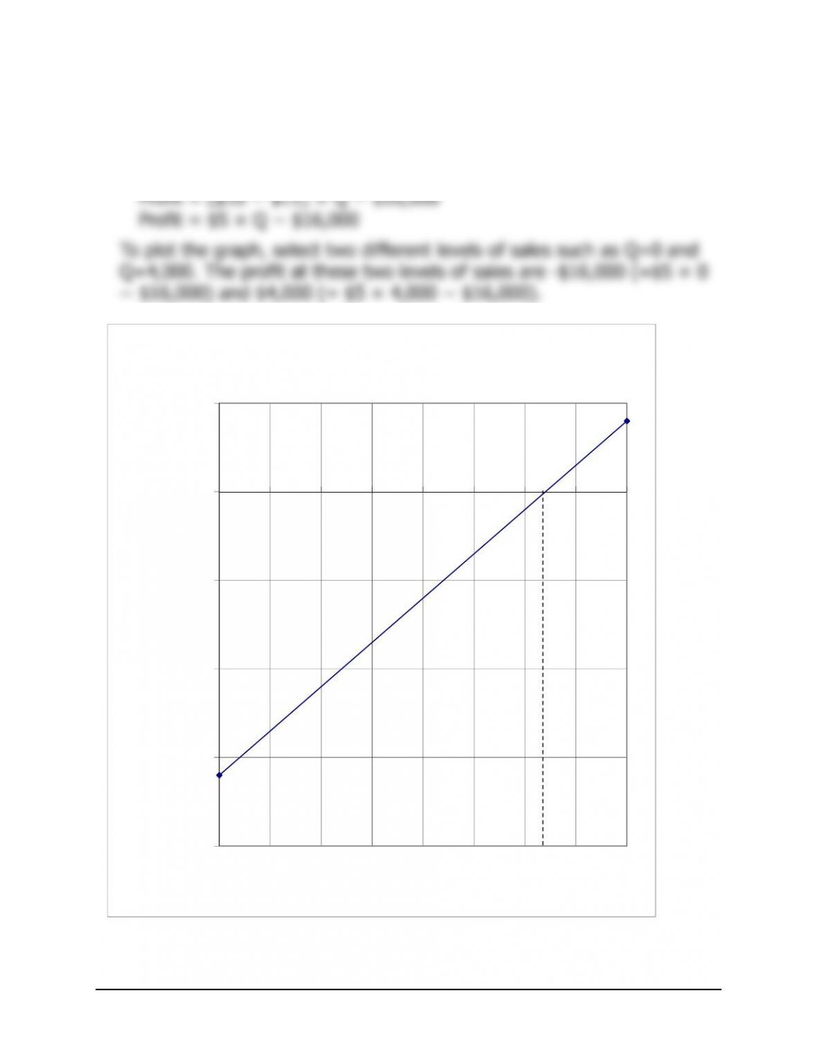
1. The CVP graph can be plotted using the three steps outlined in the text.
The graph appears on the next page.
Step 1. Draw a line parallel to the volume axis to represent the total
Step 2. Choose some volume of sales and plot the point representing
total expenses (fixed and variable) at the activity level you have
Step 3. Choose some volume of sales and plot the point representing
total sales dollars at the activity level you have selected. We’ll use the
2. The break-even point is the point where the total sales revenue and the
total expense lines intersect. This occurs at sales of 4,000 units. This
can be verified as follows:
© The McGraw-Hill Companies, Inc., 2018. All rights reserved.
18 Managerial Accounting, 16th Edition
Exercise 5-2 (continued)
$0
$50,000
$100,000
$150,000
$200,000
0 2,000 4,000 6,000 8,000
Dollars
Volume in Units
CVP Graph
© The McGraw-Hill Companies, Inc., 2018. All rights reserved.
Solutions Manual, Chapter 5 19
Exercise 5-3 (15 minutes)
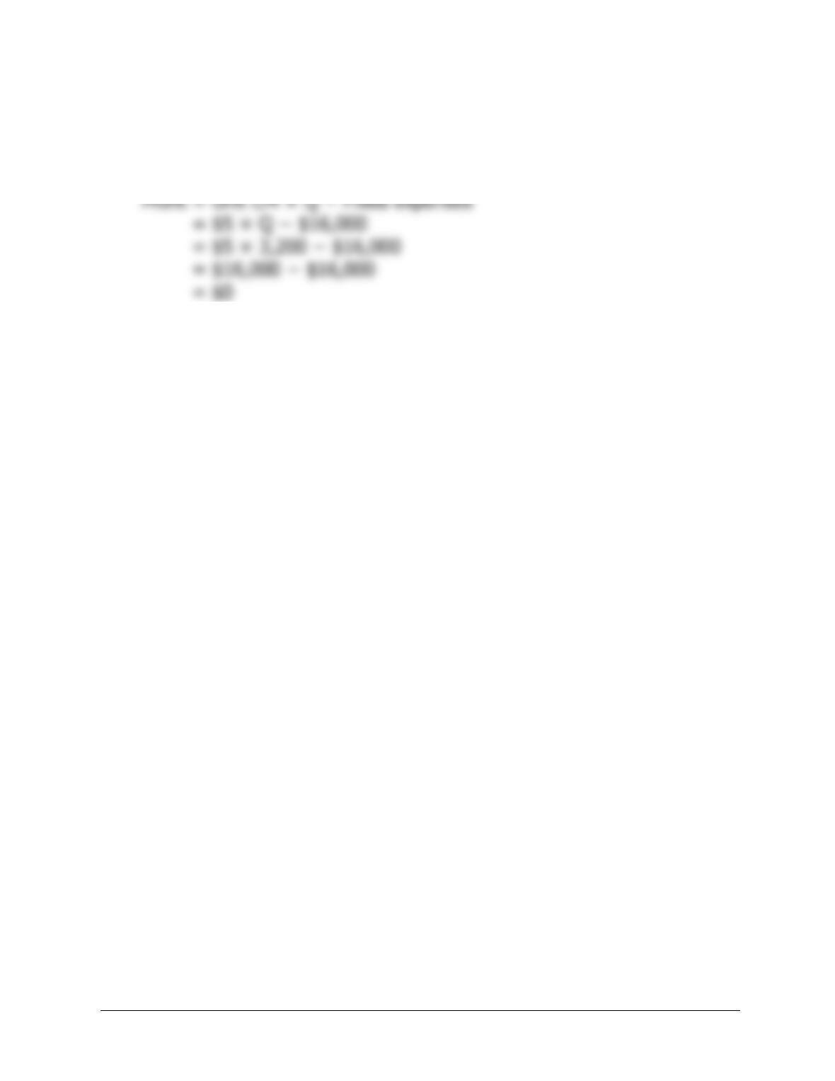
1. The profit graph is based on the following simple equation:
Profit = Unit CM × Q − Fixed expenses
-$20,000
-$15,000
-$10,000
-$5,000
$0
$5,000
0 500 1,000 1,500 2,000 2,500 3,000 3,500 4,000
Profit
Sales Volume in Units
Profit Graph
© The McGraw-Hill Companies, Inc., 2018. All rights reserved.
20 Managerial Accounting, 16th Edition
Exercise 5-3 (continued)
2. Looking at the graph, the break-even point appears to be 3,200 units.
This can be verified as follows: