978-1260152616 Appendix APPENDIX E

Unlock access to all the studying documents.

View Full Document

Appendix E – Using Indifference Curves

APPENDIX E

USING INDIFFERENCE

CURVES

Learning Objectives

LO E.1: Explain how the marginal rate of substation relates to the shape of

the indifference curve.

LO E.2: Outline the four properties that apply to all indifference curves.

LO E.3: Explain the shapes of indifference curves for perfect substitutes and

perfect complements.

LO E.4: Describe the point at which a consumer maximized utility.

LO E.5: Show how changes in income and prices affects utility maximization.

LO E.6: Show how to build an individual’s demand curve using indifference

curves.

Appendix Outline

Representing Preferences Graphically

Consumption bundles and indifference curves (LO E.1)

Properties of indifference curves (LO E.2)

Perfect substitutes and perfect complements (LO E.3)

Understanding Consumer Choice

Equalizing the marginal utility of the last purchase (LO E.4)

Finding the highest indifference curve

How Consumers Respond to Change (LO E.5)

Responding to a change in income

Responding to a change in prices

Deriving the demand curve using the indifference curves (LO E.6)

Review Questions

1. If an indifference curve is a vertical line, does the amount of the good

on the y-axis influence the consumer’s utility? [LO E.1]

Answer: Here, marginal rate of subsitution is zero or undefined. A vertical

indifference curve means that the utility or satisfaction derived from

consuming any small or large quantity of the good whose consumption is

E-1

Education.

Appendix E – Using Indifference Curves

2. Two friends are discussing their plans for the month. One works at a

movie theater and gets 10 free movie tickets; the other works at a concert

venue and gets 10 free concert tickets. What can we predict about the first

person’s marginal rate of substitution between movies and concerts? What

can we predict about the second person’s marginal rate of substitution

between the two? How does this relate to the slope of each of their

indifference curves? [LO E.1]

Answer: If both goods are perfect substitutes where each person is

indifferent between a movie and a concert, the MRS = 1 and the slope has

3. Your good friend tells you that althought she has a large amount of

M&Ms and just a few Skittles, she would still be willing to give you the rest of

her Skittles, just to get one last M&M. What characteristic of indifference

curves is your friend going against? [LO E.2]

Answer: Typically with normal goods, as we consume more of a good, the

marginal utility of the good decreases. Since your friend has many M&Ms and

4. For each pair of goods listed below, state whether the indifference

curves would be linear or L-shaped. [LO E.3]

Ten dollar bills and pairs of 9ve dollar bills.

Coffee and tea.

Bagels and muJns.

Left shoes and right shoes.

Answer: Left shoes and right shoes; The graph shows indifference curves

5. Suppose that a budget constraint intersects an indifference curve at

two separate points. Can either of these consumption bundles be optimal?

Explain why or why not. [LO E.4]

E-2

Education.

Appendix E – Using Indifference Curves

Answer: The optimal consumption bundle occurs where the budget line is

6. Dan consumes two goods: peanut butter and jelly sandwiches, which

are an inferior good, and chicken salad sandwiches, which are a normal

good. He gets a raise at work. Will the ratio of peanut butter and jelly

sandwiches to chicken salad sandwiches that he consumes increase or

decrease? [LO E.5]

Answer: Assuming that the ratio of consumption is [quantity of peanut

7. Haley divides her entertainment budget between movie tickets and

concert tickets. Two of her indifference curves are shown in Figure EQ-1.

When movie tickets are $12 and concert tickets are $20, she purchases 25

movie tickets and 45 concert tickets. This is shown on Indifference Curve 1

(IC1). Haley 9nds out that she can sign up for a loyalty program with the

movie theater and buy tickets at a 50% discount. When the price of movie

tickets decreases, she buys 50 movie tickets and 50 concert tickets. This is

shown on Indifference Curve 2 (IC2). For which of these two goods can we

draw Haley’s demand curve? Explain. [LO E.6]

Answer: The demand curve describes how the quantity demanded of a

For movie tickets, we now have two different prices and two different

quantities demanded. This is all we need to draw a demand curve.

Problems and Applications

1. Your baby cousin Hubert loves lollipops and bouncy balls. Look at the

indifference curves in Figure EP-1 that represent his preferences among

various bundles of the two goods. Assuming the indifference curves follow

the four properties outlined in this appendix, rank bundles A through D from

the highest utility to the lowest, including ties. [LO E.1]

Answer: Bundle A: Lowest utility

E-3

Education.

Appendix E – Using Indifference Curves

Each point on each of the curves represents a consumption bundle that

gives Hubert the same amount of satisfaction as the other bundles on

that curve. If his consumption moves from point D on curve Ib to point C,

2. Table EP–1 shows some possible consumption bundles for a person who

consumes MP3s and lattes. [LO E.2]

a. Which bundles fall on the lowest indifference curve?

b. Which bundles fall on the highest indifference curve?

Answer: The bundle on the lowest indifference curve is the one with the

3. Determine whether the preferences described below would be

represented by an indifference curve that is L-shaped, bows inwards, or is a

straight line. [LO E.2]

a. Edgar will eat carrots only if he has hummus to go with them.

b. Andrew likes to start his day right with oatmeal, but he’s just as

happy starting it with steel-cut oats as he is with rolled oats.

c. Ezekiel really enjoys coffee and donuts together, but he’s also happy

eating just one of the other.

Answer: Perfect complements are useless without the other good. The

Since steel-cut oats and rolled oats are perfect substitutes, Andrew is

willing to trade one for the other in order to maintain the same amount of

An indifference curve shows all of the options between which a consumer

is truly indifferent. By “indifferent,” economists don’t mean that the

E-4

Education.

Appendix E – Using Indifference Curves

4. Jonah is completely indifferent between eating the brand name version

of his favorite cereal and eating the generic version. His preferences would

best be represented by which indifference curve on Figure EP-2: ICa or ICb?

Are brand-name cereal of generic cereal perfect substitutes or perfect

complements?

Answer: If Jonah is completely indifferent between brand-name and

5. A consumer is stocking up on sodas and sports drinks at the dollar

store. As you might expect as a dollar store, each bottles of each drink costs

$1. He has a $10 bill to spend. Based on Table EP-2 of marginal utilities, 9nd

the optimal consumption bottle. [LO E.4]

Answer: At the optimal consumption bundle, the slope of the budget line

is the same as the slope of the indifference curve—they are tangent to

one another. Optimal consumption occurs at the point where the marginal

6. A consumer is buying steaks for $4 each potatoes for $1 per pound.

She has $40. Plot her budget constraint on Figure EP-3 and 9nd her optimal

consumption bundle. [LO E.4]

Answer: At the optimal consumption bundle, the slope of the budget line

is the same as the slope of the indifference curve—they are tangent to

E-5

Education.

Appendix E – Using Indifference Curves

7. Under utility maximization, is it possible that after an increase in

income, a consumer would remain on the same indifference curve? What

about after a decrease in the price of one of the goods? [LO E.5]

Answer: An increase in income leads to more consumption as long as

both goods are normal, meaning that the consumer demands more of

Depending on the type of good, the income and substitution effects will

have different impacts on the optimal consumption bundle of the

8. True or false? The income effect is represented by the shift in

consumption of a good as a bundle moves along the old indifference curve

before moving to another indifference curve tangent to the new budget line.

[LO E.5]

Answer: False. Consumption shifts up to the highest indifference curve

that is now accessible due to the increase in purchasing power (income

effect). Consumption responds to the changes in relative prices

9. Tyler likes to divide his entertainment between attending basketball

games and attending football games. Two of his indifference curves are

shown in Figure EP-4. When football games are $25 and basketball games

are $20, he chooses to attend 6 football games and 7 basketball games. This

is shown in Indifference Curve 1 (IC1). The football team has been selling out

every game, so they decide to raise the price to $45 a per game. At this new

price, Tyler chooses to attend 2 football games and 8 basketball games. This

is shown on Indifference Curve 2 (IC2). [LO E.6]

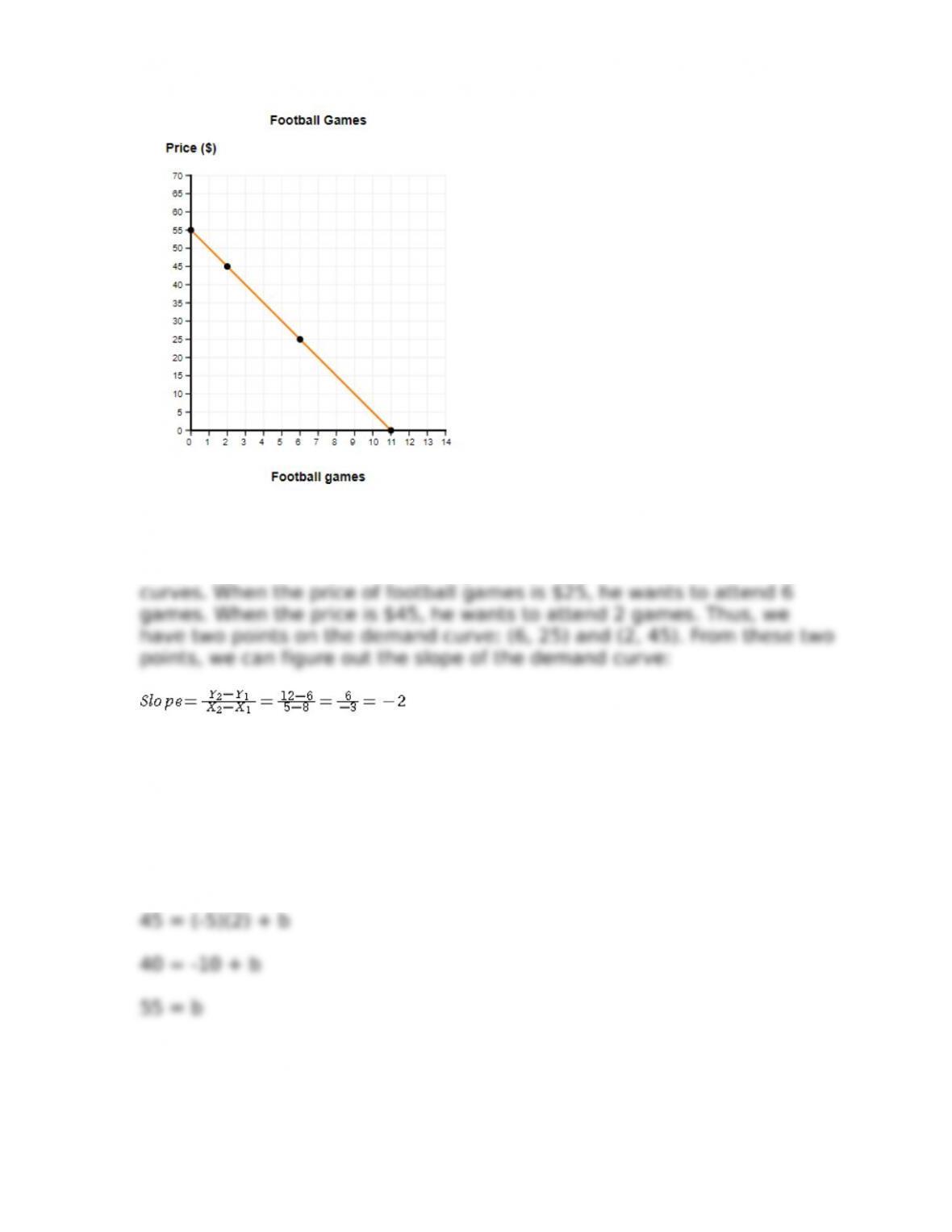
a. Draw Tyler’s demand curve for football games.

b. What is the slope of the Tyler’s demand curve for football games?

Answer: a.

E-6

Education.

Appendix E – Using Indifference Curves

b. The slope of Tyler’s demand curve for football games is -5.

We plot Tyler’s demand curve using information from his indifference

Using the slope, we can determine the x- and y-intercepts.

The equation of a line is Y = mX + b, where m is the slope and b is the y-

intercept. We can plug in the slope and one of our known points to 9nd

the y-intercept. Let’s use (2, 45):

Y = mX + b

This tells us the y-intercept is (0, 55). Now, we can use the slope, the y-

intercept, and a y value of zero to 9nd the x-intercept:

E-7

Education.

Appendix E – Using Indifference Curves

Thus, the x-intercept is (11, 0).

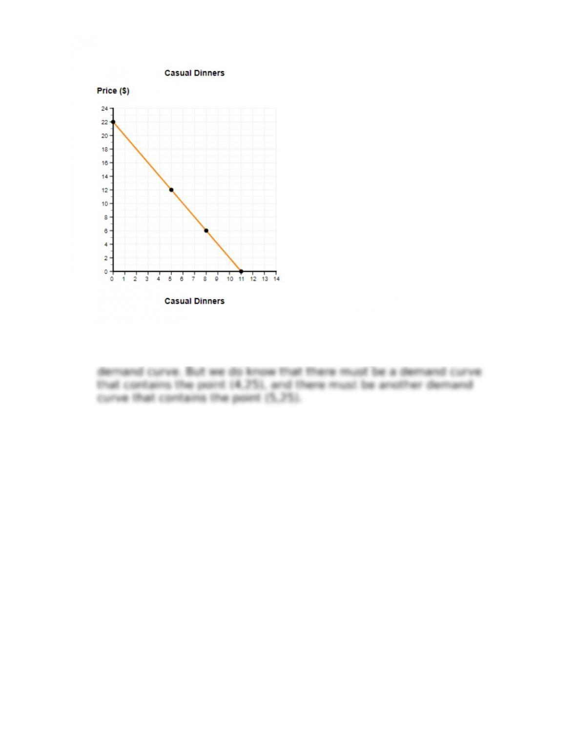
10. Gabriella divides her food budget between fancy dinners and

casual dinners. Two of her indifference curves are shown in Figure EP-5.

When casual dinners are $12 and fancy dinners are $25, she chooses 5

casual dinners and 4 fancy dinners. This is shown in Indifference Curve 1

(IC1). A new restaurant opens near her apartment, and she can get a casual

dinner for $6. At this new price, she chooses 8 casual dinners and 5 fancy

dinners. This is shown on Indifference Curve 2 (IC2). [LO E.6]

a. Draw Gabriella’s demand curve for casual dinners.

b. What do we know about Gabriella’s demand for fancy dinners?

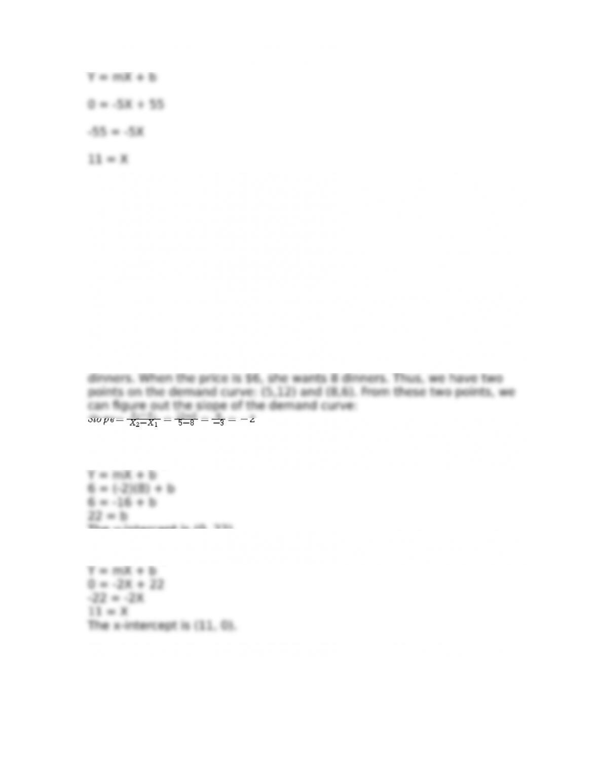
Answer: a. We plot Gabriella’s demand curve using information from her

indifference curves. When the price of casual dinners is $12, she wants 5

Using the slope, we can determine the x- and y-intercepts. The equation

of a line is Y = mX + b. We can use one of the known points to calculate

the y-intercept:

The y-intercept is (0, 22).

Now we can use the slope, the y-intercept, and a y-value of zero to 9nd

the x-intercept:

E-8

Education.

Appendix E – Using Indifference Curves

b. We don’t know much about Gabriella’s demand for fancy dinners.

Because the price of fancy dinners did not change, we cannot plot the

E-9

Education.