Appendix B – Math Essentials: Working with Linear Equations
APPENDIX B
MATH ESSENTIALS:
WORKING WITH
LINEAR EQUATIONS
Learning Objectives
LO B.1: Use linear equations to interpret the equation of a line.
LO B.2: Use linear equations to explain shifts and pivots.
LO B.3: Use linear equations to solve for equilibrium.
Appendix Outline
Interpreting the Equation of a Line (LO B.1)
Turning the graph into an equation
Turning the equation into a graph
Equations with x and y reversed
Shifts and Pivots (LO B.2)
Solving for Equilibrium (LO B.3)
Problems and Applications
1. Use the demand curve in Figure BP-1 to derive a demand equation. [LO
B.1]
Answer: First, use the endpoints to calculate the slope. The slope is the
To 3nd the Y–intercept, look at the graph and determine where the line
2. Use the demand schedule in Table BP-1 to derive a demand equation.
[LO B.1]
Answer: The y-intercept occurs where quantity demanded = 0, or 80.
B-1
Copyright © 2018 McGraw-Hill Education. All rights reserved. No reproduction or distribution without the prior written consent of McGraw-Hill
Education.
Appendix B – Math Essentials: Working with Linear Equations
3. Use the supply curve in Figure BP-2 to derive a supply equation. [LO
B.1]
Answer: The y-intercept occurs where the line crosses the y–axis, which
4. Use the supply schedule in Table BP-2 to derive a supply equation.
[ [LO B.1]
Answer: The y-intercept occurs where quantity supplied = 0, or 100. The
5. Graph the equation P = 2Q + 3. Is this the supply curve or demand
curve? [LO B.1]
Answer: This line slopes upward, so it is a supply curve. The slope is the
6. Graph the equation P = -8Q + 10. Is this the supply curve or demand
curve? [LO B.1]
Answer: This line slopes downward, so it is a demand curve. The slope is
7. Rearrange the equation Q = 5 – 0.25P and sketch the graph. Is this a
supply curve or a demand curve? [LO B.1]
Answer: Start with Q = 5 – 0.25P. Subtract 5 from both sides: Q – 5 = –
8. Rearrange the equation Q = 0.2P and sketch the graph. Is this a supply
curve or a demand curve? [LO B.1]
Answer: Start with Q = 0.2P. Divide both sides by 0.2: 5Q = P. Re-
B-2
Copyright © 2018 McGraw-Hill Education. All rights reserved. No reproduction or distribution without the prior written consent of McGraw-Hill
Education.
Appendix B – Math Essentials: Working with Linear Equations
9. The entrance fee at your local amusement park is $20 for the day. The
entrance fee includes all rides except roller coasters. Roller coasters cost an
extra $2 per ride. [LO B.2]
a. Write an equation that represents how much money you will spend
on rides as a function of the number of rides you on: S = total
spending on rides; Q = the quantity of roller coasters rides.
b. What is your total spend on rides if you ride 4 roller coasters?
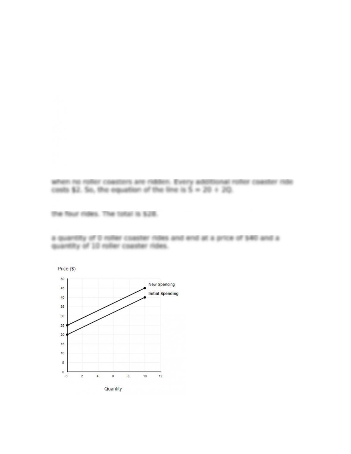
c. Draw a graph of the relationship between total spending on rides
and the number of roller coaster rides.
d. Redraw the graph from part (c) to show what changes if the
entrance fee increases to $25.
e. Rewrite the equation from part (a) to incorporate the increased
entrance fee of $25.
f. After the entrance fee increases to $25, what is your total spending
on rides if you ride 4 roller coasters?
Answer: a. The y-intercept is 20, which is the cost of the entrance fee
c. See the correct graph below. The line should start at a price of $20 and
B-3
Copyright © 2018 McGraw-Hill Education. All rights reserved. No reproduction or distribution without the prior written consent of McGraw-Hill
Education.
Appendix B – Math Essentials: Working with Linear Equations
d. If the entrance fee increases to $25, the line will shift up by $5, but will
e. Since the entrance fee is all that has changed, only the y-intercept
f. If you ride 4 roller coasters, you will pay $25 for entry plus $2 × 4 for
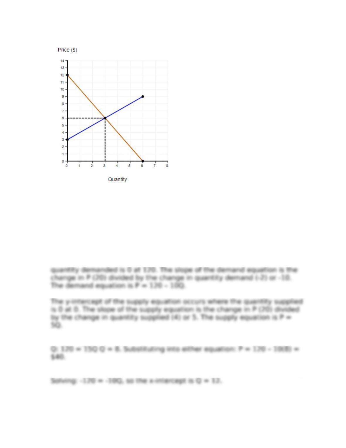
10. Use the following two equations: [LO B.3]
(1) P = 12 – 2Q
(2) P = 3 +Q
a. Find the equilibrium price and quantity.
b. Graph the demand and supply equations. Illustrate the equilibrium
point.
Answer:
a. Setting the equations equal to each other: 12 – 2Q = 3+ Q. Solving for
The x-intercept for the demand line occurs where P = 0. So 0 = 12 – 2Q.
The y-intercept for the demand line occurs where Q = 0. So the y–
The endpoint for the supply line is determined where Q = 6. So when Q =
B-4
Copyright © 2018 McGraw-Hill Education. All rights reserved. No reproduction or distribution without the prior written consent of McGraw-Hill
Education.
Appendix B – Math Essentials: Working with Linear Equations
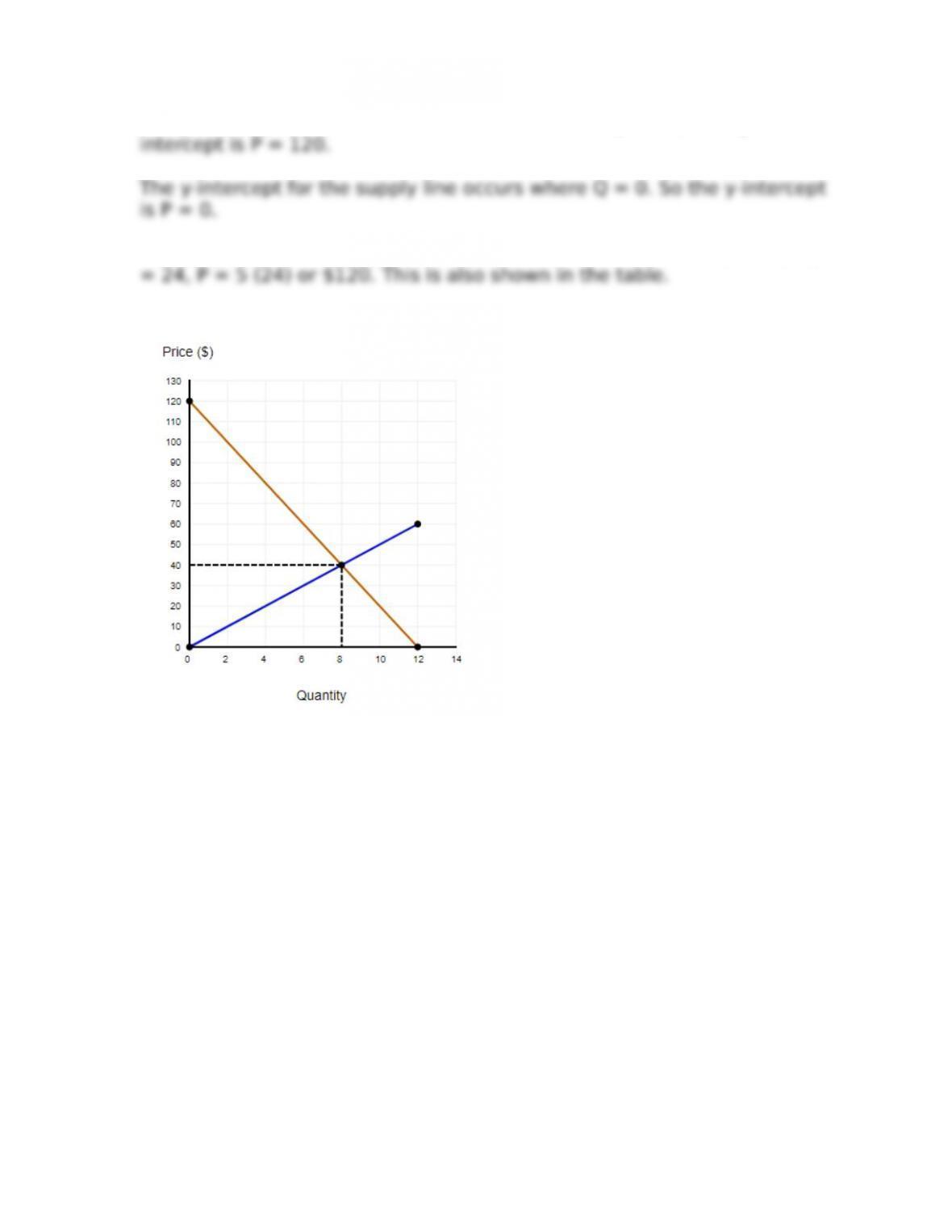
11. With reference to Table BP-3: [LO B.3]
a. Use the information from the table to create the demand and supply
equations.
b. Use your demand and supply equations to solve for equilibrium.
c. Graph supply and demand curves. Illustrate the equilibrium point.
Answer: a. The y-intercept of the demand equation occurs where the
b. Setting the equations equal to each other: 120 – 10Q = 5Q. Solving for
The x-intercept for the demand line occurs where P = 0. So 0 = 120 – 10Q.
B-5
Copyright © 2018 McGraw-Hill Education. All rights reserved. No reproduction or distribution without the prior written consent of McGraw-Hill
Education.
Appendix B – Math Essentials: Working with Linear Equations
The y-intercept for the demand line occurs where Q = 0. So the y–
The endpoint for the supply line is determined where Q = 24. So when Q
c.
B-6
Copyright © 2018 McGraw-Hill Education. All rights reserved. No reproduction or distribution without the prior written consent of McGraw-Hill
Education.