Chapter 06 – Efficient Diversification
CHAPTER 06
EFFICIENT DIVERSIFICATION
1. So long as the correlation coefficient is below 1.0, the portfolio will benefit from
3. a and b will have the same impact of increasing the Sharpe ratio from .40 to .45.
4. The expected return of the portfolio will be impacted if the asset allocation is changed.
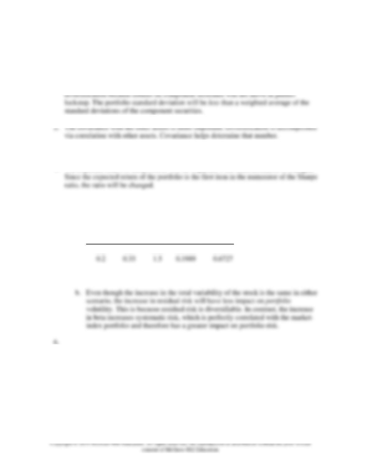
5. Total variance = Systematic variance + Residual variance = β2 Var(rM) + Var(e)
When β = 1.5 and σ(e) = .3, variance = 1.52 × .22 + .32 = .18. In the other scenarios:
sMs(e) b
TOTAL
Variance
Corr Coeff
0.2 0.3 1.65 0.1989 0.7399
0.2 0.33 1.5 0.1989 0.6727
a. Both will have the same impact. Total variance will increase from .18 to .1989.
Thus, there appears to be a higher variance, yet the mean is probably the same
since the spread is equally large on both the high and low side. The mean return,
however, should be higher since there is higher probability given to the higher
returns.
Chapter 06 – Efficient Diversification
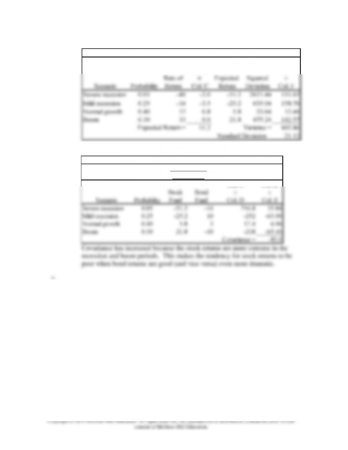
b. Calculation of mean return and variance for the stock fund:
(A) (B) (C) (D) (E) (F) (G)
Col. B
Col. B
×
Col. C
Col. F
Severe recession 0.05 –40 –2.0 –51.2 2621.44 131.07
Mild recession 0.25 –14 –3.5 –25.2 635.04 158.76
Normal growth 0.40 17 6.8 5.8 33.64 13.46
Boom 0.30 33 9.9 21.8 475.24 142.57
11.2 445.86
21.12
Scenario
Deviation
from
Expected
Return
Squared
Deviation
Expected Return =
Variance =
Standard Deviation =
Rate of
Return
Probability
c. Calculation of covariance:
(A) (B) (C) (D) (E) (F)
Col. C Col. B
Stock Bond
Fund Fund Col. D Col. E
Severe recession 0.05 –51.2 –14 716.8 35.84
Mild recession 0.25 –25.2 10 –252 –63.00
Normal growth 0.40 5.8 3 17.4 6.96
Boom 0.30 21.8 –10 –218 –65.40
Covariance = –85.6
Deviation from
Mean Return
Scenario
Probability
Covariance has increased because the stock returns are more extreme in the
recession and boom periods. This makes the tendency for stock returns to be
poor when bond returns are good (and vice versa) even more dramatic.
7. a. One would expect variance to increase because the probabilities of the extreme
outcomes are now higher.
Chapter 06 – Efficient Diversification
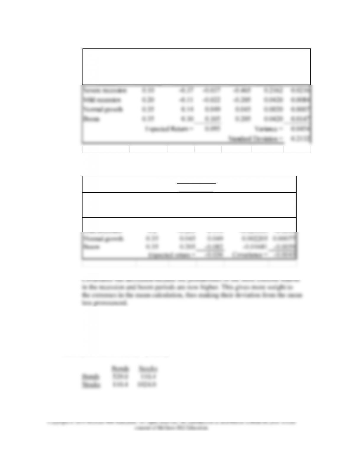
b. Calculation of mean return and variance for the stock fund:
Col. B Col. B
Col. C Col. F
Severe recession 0.10 –0.37 –0.037 –0.465 0.2162 0.0216
Mild recession 0.20 –0.11 –0.022 –0.205 0.0420 0.0084
Normal growth 0.35 0.14 0.049 0.045 0.0020 0.0007
Boom 0.35 0.30 0.105 0.205 0.0420 0.0147
0.095 0.0454
0.2132
Expected Return =
Variance =
Standard Deviation =
Scenario
Probability
Stock
Rate of
Return
Deviation
from
Expected
Return
Squared
Deviation
c. Calculation of covariance
Col. C Col. B
Stock Bond
Fund Fund Col. D Col. E
Severe recession 0.1 –0.465 –0.122 0.05673 0.00567
Mild recession 0.2 –0.205 0.119 –0.024395 –0.0049
Normal growth 0.35 0.045 0.049 0.002205 0.00077
Boom 0.35 0.205 –0.082 –0.01681 –0.0059
–0.036 Covariance = –0.0043
Deviation from
Mean Return
Scenario
Probability
Expected return =
8. The parameters of the opportunity set are:
E(rS) = 15%, E(rB) = 9%, S = 32%, B = 23%, = 0.15, rf = 5.5%
From the standard deviations and the correlation coefficient we generate the covariance
matrix [note that Cov(rS, rB) = SB]:
The minimum-variance portfolio proportions are:
Chapter 06 – Efficient Diversification
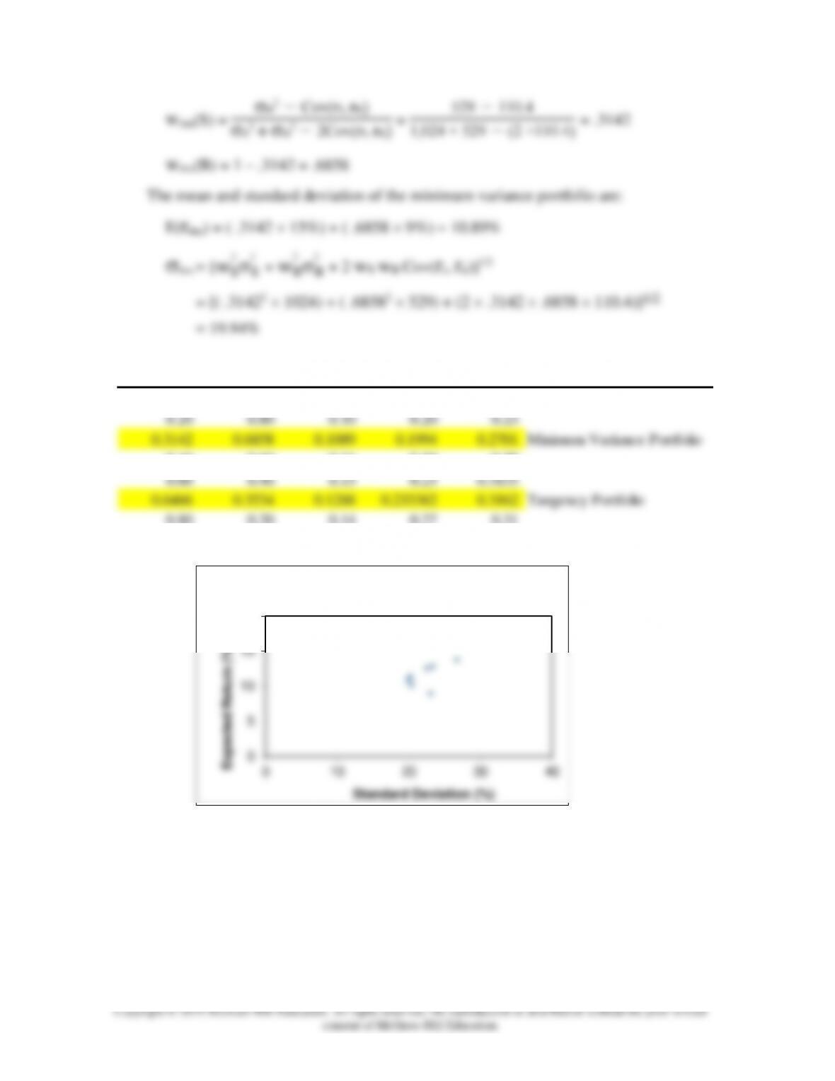
wMin(S) = B2 - Cov(rS, rB)
S2 + B2 - 2Cov(rS, rB) = 529 - 110.4
1,024 + 529 - (2 ×110.4) = .3142
wMin(B) = 1 – .3142 = .6858
The mean and standard deviation of the minimum variance portfolio are:
E(rMin) = ( .3142 15%) + ( .6858 9%) = 10.89%
Min = [wS
2S
2 + wB
2B
2 + 2 wS wB Cov(rS, rB)]1/2
= [( .31422 1024) + ( .68582 529) + (2 .3142 .6858 110.4)]1/2
= 19.94%
% in stocks % in bonds Exp. Return Std dev.
Sharpe Ratio
0.00 1.00 0.09 0.23 0.15
0.20 0.80 0.10 0.20 0.23
0.3142 0.6858 0.1089 0.1994 0.2701 Minimum Variance Portfolio
0.40 0.60 0.11 0.20 0.29
0.60 0.40 0.13 0.23 0.3155
0.6466 0.3534 0.1288 0.233382 0.3162 Tangency Portfolio
0.80 0.20 0.14 0.27 0.31
1.00 0.00 0.15 0.32 0.30
0
5
10
15
20
010 20 30 40
Expected Return (%)
Standard Deviation (%)
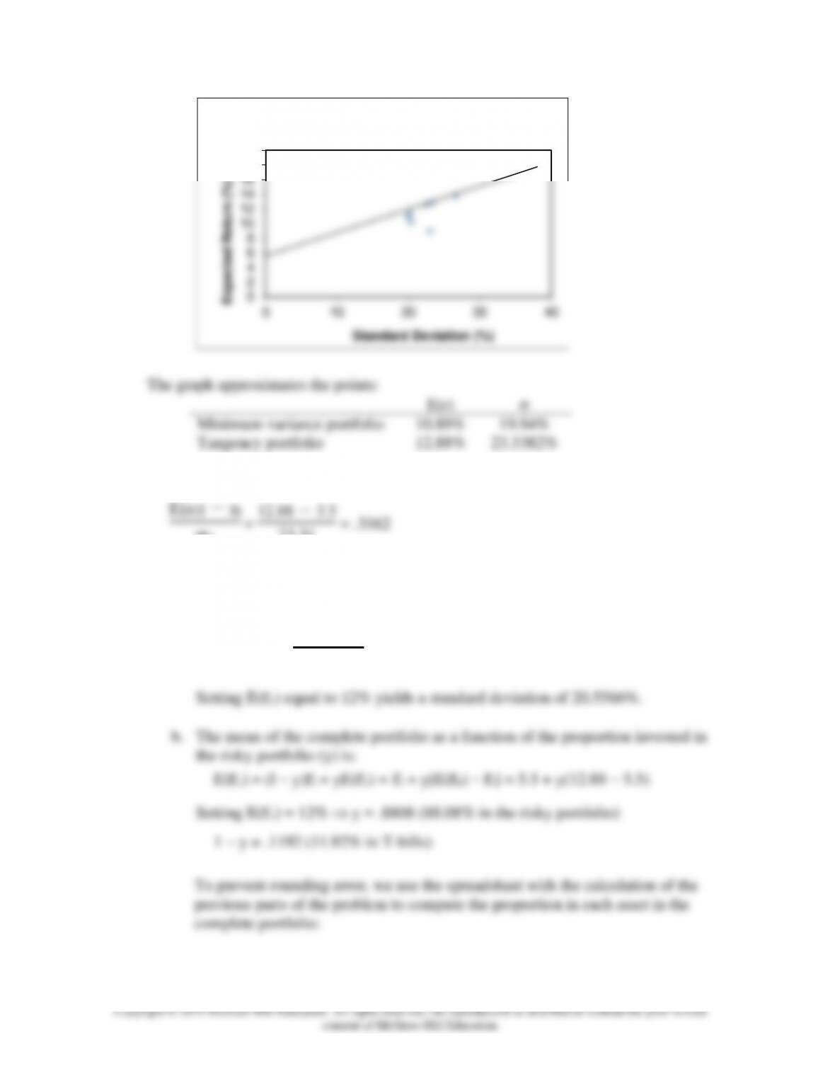
Investment Opportunity Set
Chapter 06 – Efficient Diversification
The graph approximates the points:
E(r)
Minimum variance portfolio
10.89%
19.94%
Tangency portfolio
12.88%
23.3382%
10. The Sharpe ratio of the optimal CAL is:
P
23.34 = .3162
11.
a. The equation for the CAL is:
E(rC) = rf + E(rP) - rf
P
C = 5.5 + .3162C
complete portfolio:
0
2
4
6
8
10
12
14
16
18
20
010 20 30 40
Expected Return (%)
Standard Deviation (%)
Investment Opportunity Set
Chapter 06 – Efficient Diversification
(c) 0.205559955 = (12% – 5.5%)/Sharpe ratio(risky portfolio)
W(risky portfolio) 0.880786822
= (c)/(risky portfolio)
Proportion of stocks in complete portfolio
W(s) = W(risky portfolio)*% in stock of the risky portfolio
= 0.569541021
Proportion of bonds in complete portfolio
W(b) = W(risky portfolio)*% in bonds of the risky portfolio
= 0.311245801
12. Using only the stock and bond funds to achieve a mean of 12%, we solve:
12 = 15wS + 9(1 −wS ) = 9 + 6wS wS = .5
13.
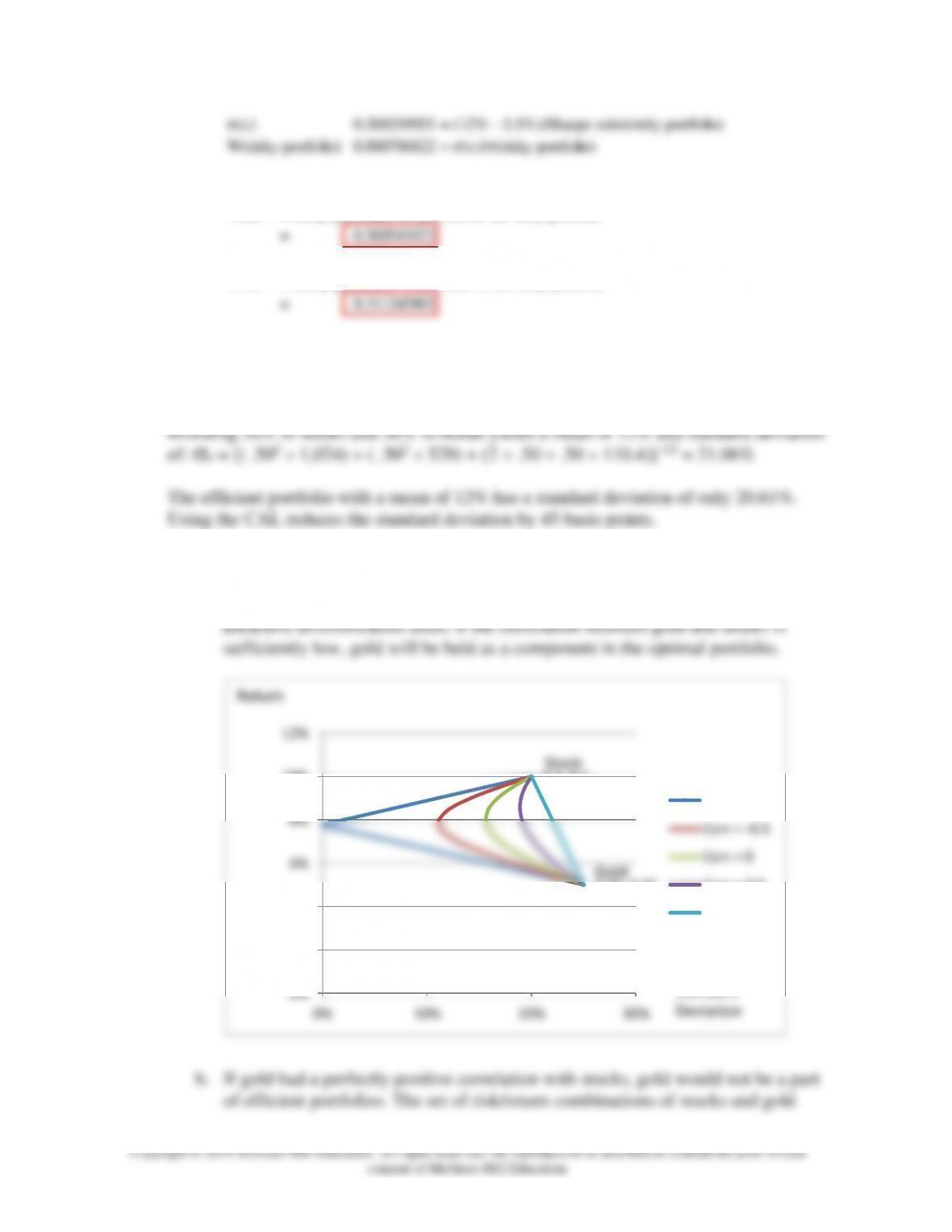
a. Although it appears that gold is dominated by stocks, gold can still be an
Copyright © 2019 McGraw-Hill Education. All rights reserved. No reproduction or distribution without the prior written
consent of McGraw-Hill Education.
14. Since Stock A and Stock B are perfectly negatively correlated, a risk-free portfolio can
be created and the rate of return for this portfolio in equilibrium will always be the risk-
free rate. To find the proportions of this portfolio [with wA invested in Stock A and wB
15. Since these are annual rates and the risk-free rate was quite variable during the sample
period of the recent 20 years, the analysis has to be conducted with continuously
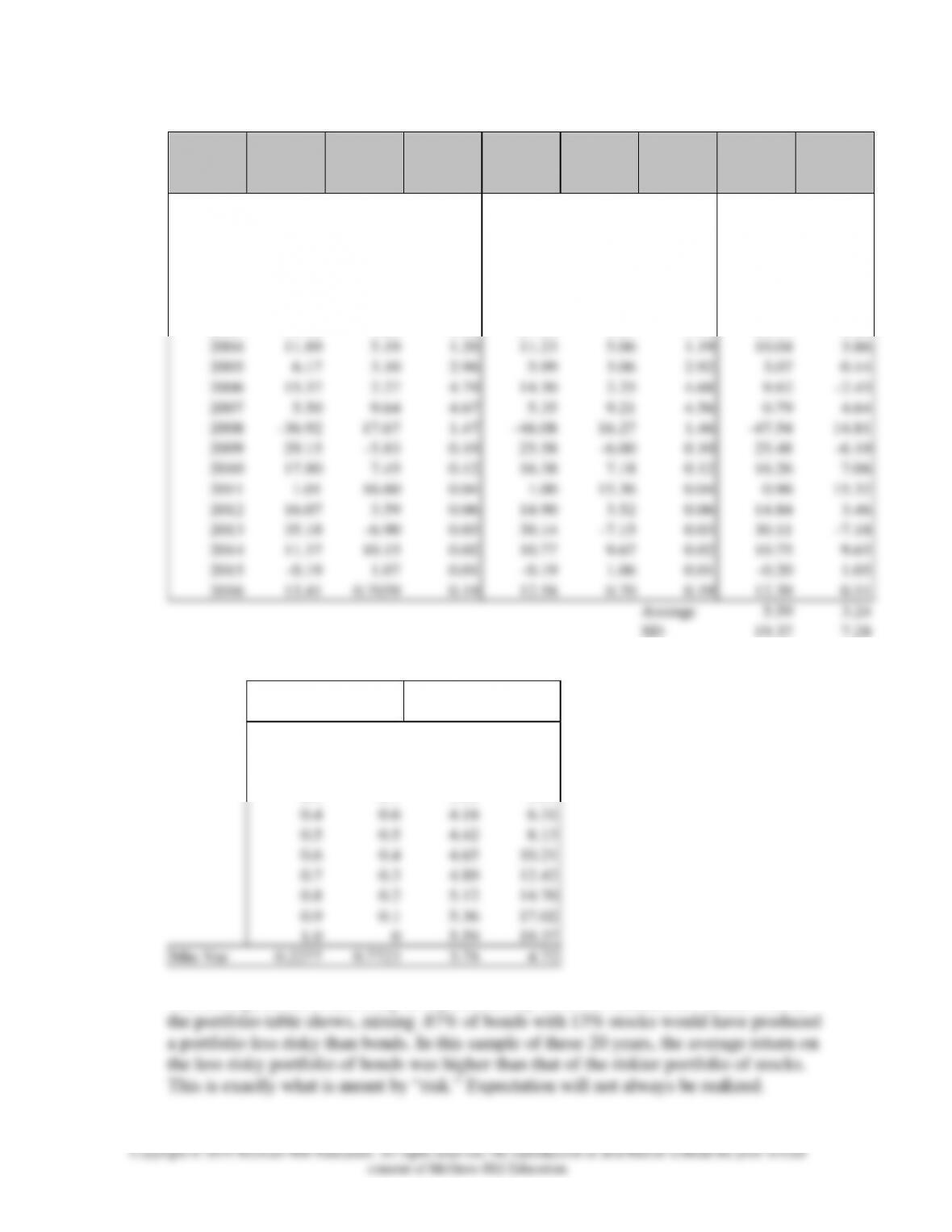
Chapter 06 – Efficient Diversification
Annual returns from Table 2 Continuously compounded rates Excess returns
Year
Large
Stock
Long-
Term T-
Bonds
T-Bills
Large
Stock
Long-
Term T-
Bonds
T-Bills
Large
Stock
Long-
Term T-
Bonds
1997 31.33 11.31 5.26 27.25 10.72 5.13 22.13 5.59
1998 24.27 13.09 4.86 21.73 12.30 4.75 16.98 7.56
1999 24.89 –8.47 4.68 22.23 –8.85 4.57 17.65 –13.43
2000 –10.82 14.49 5.89 –11.45 13.53 5.72 –17.17 7.81
2001 –11.00 4.03 3.78 –11.65 3.95 3.71 –15.36 0.24
2002 –21.28 14.66 1.63 –23.93 13.68 1.62 –25.54 12.07
2003 31.76 1.28 1.02 27.58 1.27 1.01 26.57 0.25
2004 11.89 5.19 1.20 11.23 5.06 1.19 10.04 3.86
2005 6.17 3.10 2.96 5.99 3.06 2.92 3.07 0.14
2006 15.37 2.27 4.79 14.30 2.25 4.68 9.62 –2.43
2007 5.50 9.64 4.67 5.35 9.21 4.56 0.79 4.64
2008 –36.92 17.67 1.47 –46.08 16.27 1.46 –47.54 14.81
2009 29.15 –5.83 0.10 25.58 –6.00 0.10 25.48 –6.10
2010 17.80 7.45 0.12 16.38 7.18 0.12 16.26 7.06
2011 1.01 16.60 0.04 1.00 15.36 0.04 0.96 15.32
2012 16.07 3.59 0.06 14.90 3.52 0.06 14.84 3.46
2013 35.18 –6.90 0.03 30.14 –7.15 0.03 30.11 –7.18
2014 11.37 10.15 0.02 10.77 9.67 0.02 10.75 9.65
2015 –0.19 1.07 0.01 –0.19 1.06 0.01 –0.20 1.05
2016 13.41 0.7039 0.19 12.58 0.70 0.19 12.39 0.51
0.9 0.1 5.36 17.02
1.0 05.59 19.37
Min–Var 0.2277 0.7723 3.78 4.72
The bond portfolio is less risky as represented by its lower standard deviation. Yet, as
16. If the lending and borrowing rates are equal and there are no other constraints on
portfolio choice, then the optimal risky portfolios of all investors will be identical.
were 1.0, the frontier would be a straight line connecting A and B.
18. In the special case that all assets are perfectly positively correlated, the portfolio
standard deviation is equal to the weighted average of the component-asset standard
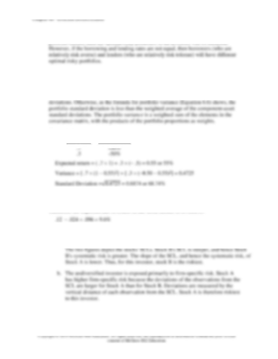
Probability
Rate of Return
.7
100%
.3
-50%
Expected return = ( .7 1) + .3 (− .5) = 0.55 or 55%
Variance = [ .7 (1 − 0.55)2] + [ .3 (−50 − 0.55)2] = 0.4725
Standard Deviation =√0.4725 = 0.6874 or 68.74%
20. The expected rate of return on the stock will change by beta times the unanticipated
change in the market return: 1.2 ( .08 – .10) = –2.4%
Therefore, the expected rate of return on the stock should be revised to:
21.
a. The risk of the diversified portfolio consists primarily of systematic risk. Beta
measures systematic risk, which is the slope of the security characteristic line (SCL).
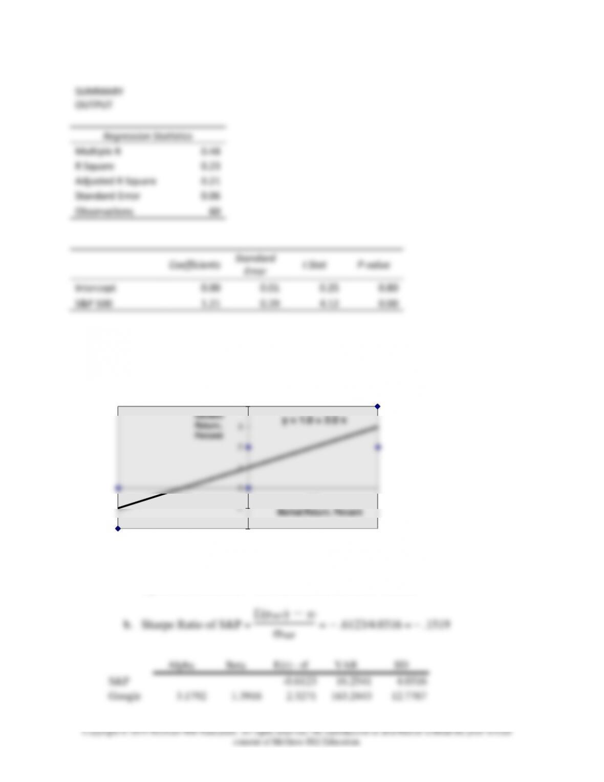
22. Using “Regression” command from Excel’s Data Analysis menu, we can run a
regression of Apple’s excess returns against those of S&P 500, and obtain the following
data. The Beta of Apple is 1.21.
Chapter 06 – Efficient Diversification
SUMMARY
OUTPUT
Regression Statistics
Multiple R
0.48
R Square
0.23
Adjusted R Square
0.21
Standard Error
0.06
Observations
60
Coefficients
Standard
Error
t Stat
P-value
Intercept
0.00
0.01
0.25
0.80
S&P 500
1.21
0.29
4.12
0.00
23. A scatter plot results in the following diagram. The slope of the regression line is 2.0
and intercept is 1.0.
y = 1.0 + 2.0 x
-2
-1
0
1
2
3
4
-1 -0.5 0 0.5 1
Market Return, Percent
Generic
Return,
Percent
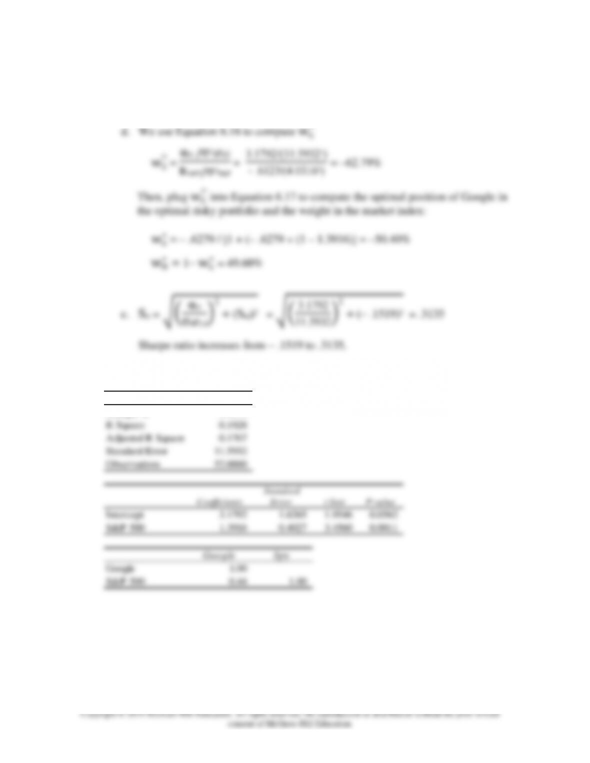
24. a. Regression output produces the following:
alpha = 3.1792, beta = 1.3916, Residual St Dev = 11.5932
Chapter 06 – Efficient Diversification
c. Information Ratio = αG/(eG) = 3.1792/11.5932 = .2742
O
O = αG /2(eG)
SUMMARY OUTPUT: Regression of Google on S&P 500 (excess returns)
Regression Statistics
Multiple R 0.4391
R Square 0.1928
Adjusted R Square 0.1767
Standard Error 11.5932
Observations 52.0000
Coefficients
Standard
Error
t Stat P-value
Intercept 3.1792 1.6265 1.9546 0.0562
S&P 500 1.3916 0.4027 3.4560 0.0011
Google Spy
Google 1.00
S&P 500 0.44 1.00
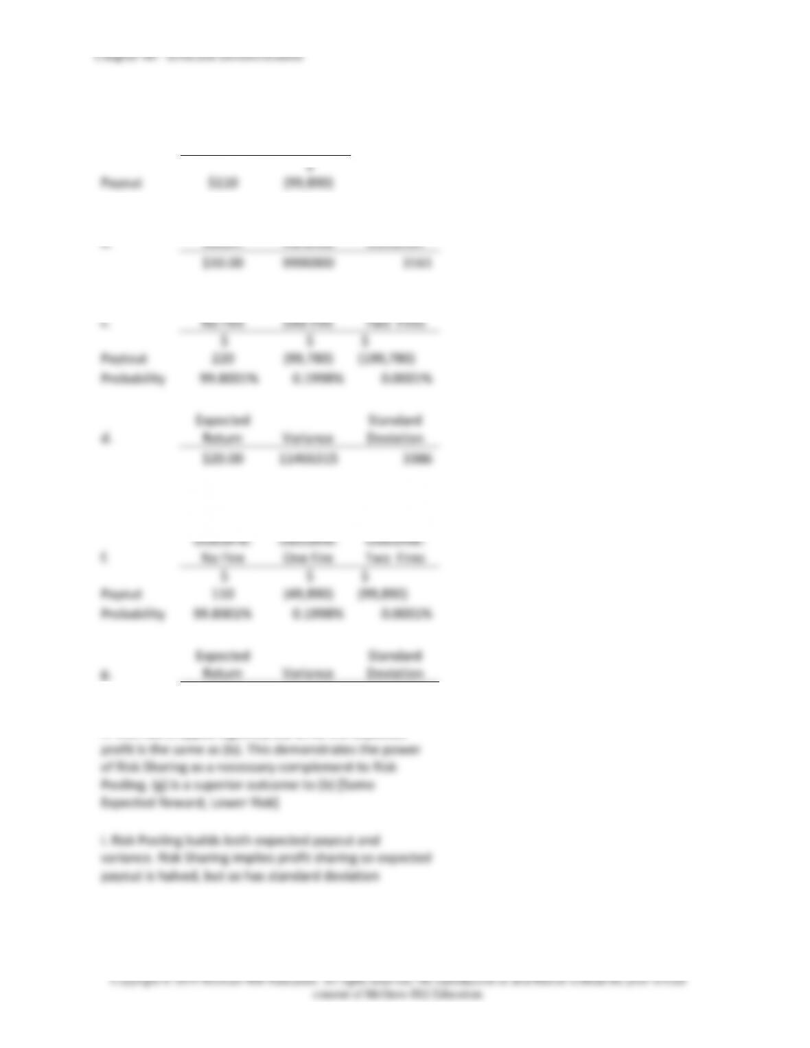
25.
a.
Outcome A:
No Fire
Outcome B:
Fire!
Payout
$110
$
(99,890)
b.
Expected
Return
Variance
Standard
Deviation
$10.00
9990000
3161
c.
Outcome:
No Fire
Outcome:
One Fire
Outcome:
Two Fires
Paytout
$
220
$
(99,780)
$
(199,780)
Probability
99.8001%
0.1998%
0.0001%
d.
Expected
Return
Variance
Standard
Deviation
$20.00
11466315
3386
e. Risk pooling increased the total variance of profit.
f.
Outcome:
No Fire
Outcome:
One Fire
Outcome:
Two Fires
Payout
$
110
$
(49,890)
$
(99,890)
Probability
99.8001%
0.1998%
0.0001%
g.
Expected
Return
Variance
Standard
Deviation
$10.00
2866579
1693
h. Risk has dropped significantly while the expected
profit is the same as (b). This demonstrates the power
of Risk Sharing as a necessary complement to Risk
Pooling. (g) is a superior outcome to (b) [Same
Expected Reward, Lower Risk]
i. Risk Pooling builds both expected payout and
variance. Risk Sharing implies profit sharing so expected
payout is halved, but so has standard deviation
Chapter 06 – Efficient Diversification
CFA 1
Answer:
CFA 2 Answer:
Fund D represents the single best addition to complement Stephenson’s current
portfolio, given his selection criteria. First, Fund D’s expected return (14.0 percent) has
the potential to increase the portfolio’s return somewhat. Second, Fund D’s relatively
CFA 3
Answer:
a. Subscript OP refers to the original portfolio, ABC to the new stock, and NP
to the new portfolio.
i. E(rNP) = wOP E(rOP ) + wABC E(rABC ) = ( .9 .67) + ( .1 1.25) = .7280%
b. Subscript OP refers to the original portfolio, GS to government securities, and
NP to the new portfolio.
Chapter 06 – Efficient Diversification
ii. CovOP , GS = CorrOP , GS OP GS = 0 2.37 0 = 0
c. Adding the risk-free government securities would result in a lower beta for the
new portfolio. The new portfolio beta will be a weighted average of the individual
security betas in the portfolio; the presence of the risk-free securities would lower
that weighted average.
d. The comment is not correct. Although the respective standard deviations and
expected returns for the two securities under consideration are identical, the
correlation coefficients between each security and the original portfolio are
CFA 4 Answer:
a. Restricting the portfolio to 20 stocks, rather than 40 to 50, will very likely
increase the risk of the portfolio, due to the reduction in diversification. Such an
increase might be acceptable if the expected return is increased sufficiently.
CFA 5
Answer:
Chapter 06 – Efficient Diversification
Risk reduction benefits from diversification are not a linear function of the number of
CFA 6
Answer:
The point is well taken because the committee should be concerned with the volatility
CFA 7
Answer:
a. Systematic risk refers to fluctuations in asset prices caused by macroeconomic
factors that are common to all risky assets; hence systematic risk is often
referred to as market risk. Examples of systematic risk factors include the
business cycle, inflation, monetary policy, and technological changes.

Chapter 06 – Efficient Diversification
Copyright © 2019 McGraw-Hill Education. All rights reserved. No reproduction or distribution without the prior written
consent of McGraw-Hill Education.
securities increases, the total risk (variance) of the portfolio approaches its
systematic variance.