Chapter 05 – Risk and Return: Past and Prologue
CHAPTER 05
RISK AND RETURN: PAST AND PROLOGUE
1. The 1% VaR will be less than –30%. As percentile or probability of a return declines so
2. If inflation increases from 3% to 5%, according to the Fisher equation there will be a
3. The excess return on the portfolio will be the same as long as you are consistent: you
can use either real rates for the returns on both the portfolio and the risk-free asset, or
4. Decrease. Typically, standard deviation exceeds return. Thus, an underestimation of 4%
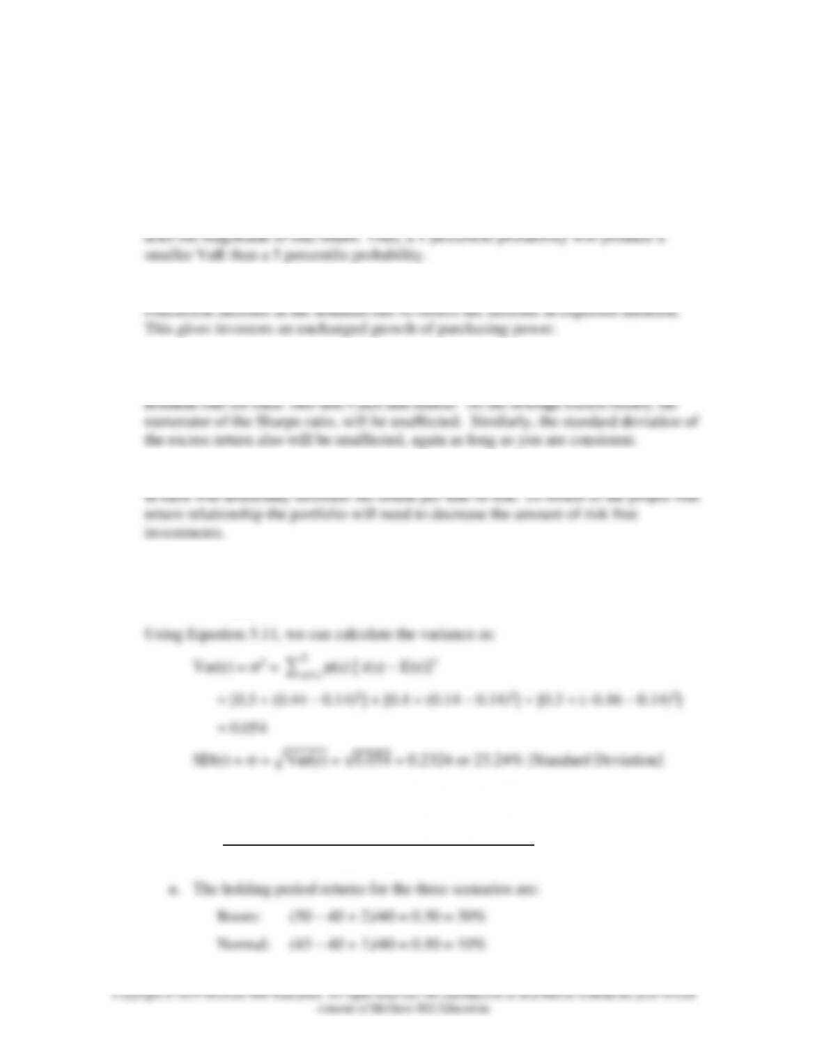
5. Using Equation 5.10, we can calculate the mean of the HPR as:
E(r) = ∑p(s) r(s)
𝑆
𝑠=1 = (0.3 0.44) + (0.4 0.14) + [0.3 (–0.16)] = 0.14 or 14%
6. We use the below equation to calculate the holding period return of each scenario:
HPR = Ending Price - Beginning Price + Cash Dividend
Beginning Price
Chapter 05 – Risk and Return: Past and Prologue
Recession: (34 – 40 + 0.50)/40 = –0.1375 = –13.75%
𝑆
b. E(r) = (0.5 8.75%) + (0.5 4%) = 6.375%
7. a. Time-weighted average returns are based on year-by-year rates of return.
Year
Return = [(Capital gains + Dividend)/Price]
2010-2011
(110 – 100 + 4)/100 = 0.14 or 14.00%
2011-2012
(90 – 110 + 4)/110 = –0.1455 or –14.55%
2012-2013
(95 – 90 + 4)/90 = 0.10 or 10.00%
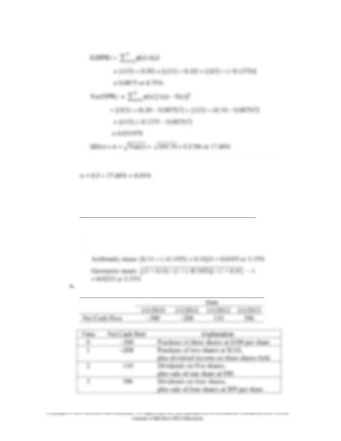
Date
1/1/2010
1/1/2011
1/1/2012
1/1/2013
Net Cash Flow
–300
–208
110
396
Time
Net Cash flow
Explanation
0
–300
Purchase of three shares at $100 per share
1
–208
Purchase of two shares at $110,
plus dividend income on three shares held
2
110
Dividends on five shares,
plus sale of one share at $90
3
396
Dividends on four shares,
plus sale of four shares at $95 per share
Chapter 05 – Risk and Return: Past and Prologue
Copyright © 2019 McGraw-Hill Education. All rights reserved. No reproduction or distribution without the prior written
consent of McGraw-Hill Education.
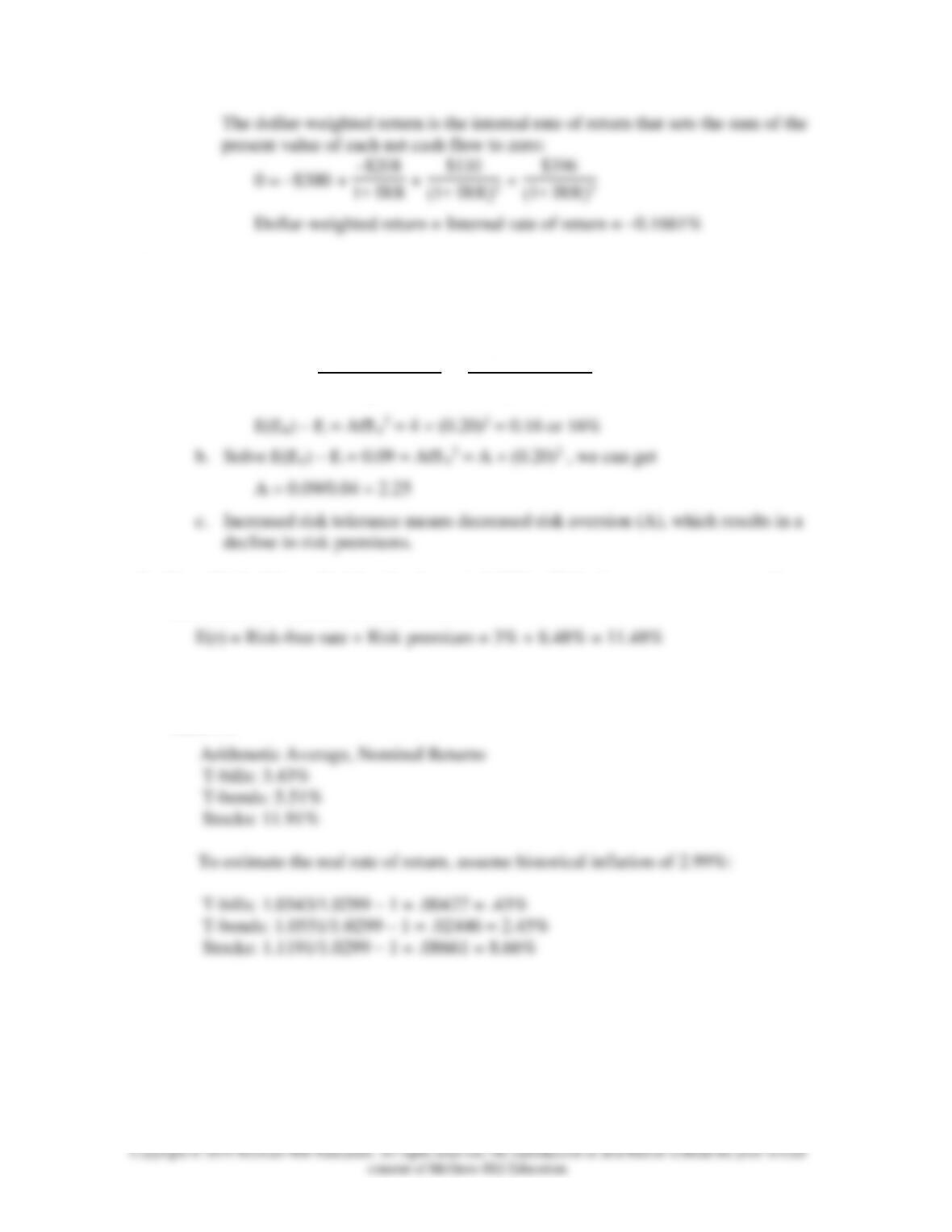
The dollar-weighted return is the internal rate of return that sets the sum of the
present value of each net cash flow to zero:
0 = –$300 + –$208
1+ IRR + $110
(1+ IRR)2 + $396
(1+ IRR)3
Dollar-weighted return = Internal rate of return = –0.1661%
8. a. Given that A = 4 and the projected standard deviation of the market return =
20%, we can use the below equation to solve for the expected market risk
premium:
A = 4 = Average(rM)- rf
Sample M2 = Average(rM)- rf
(20%)2
9. From Table 5.3, we find that for the period 1926 – 2016, the mean excess return for
S&P 500 over 1-month T-bills is 8.48%.
10. To answer this question with the data provided in the textbook, we look up the
historical average for Treasury Bills, Treasury Bonds and stocks for 1926-2016 from
Table 5.3
11.
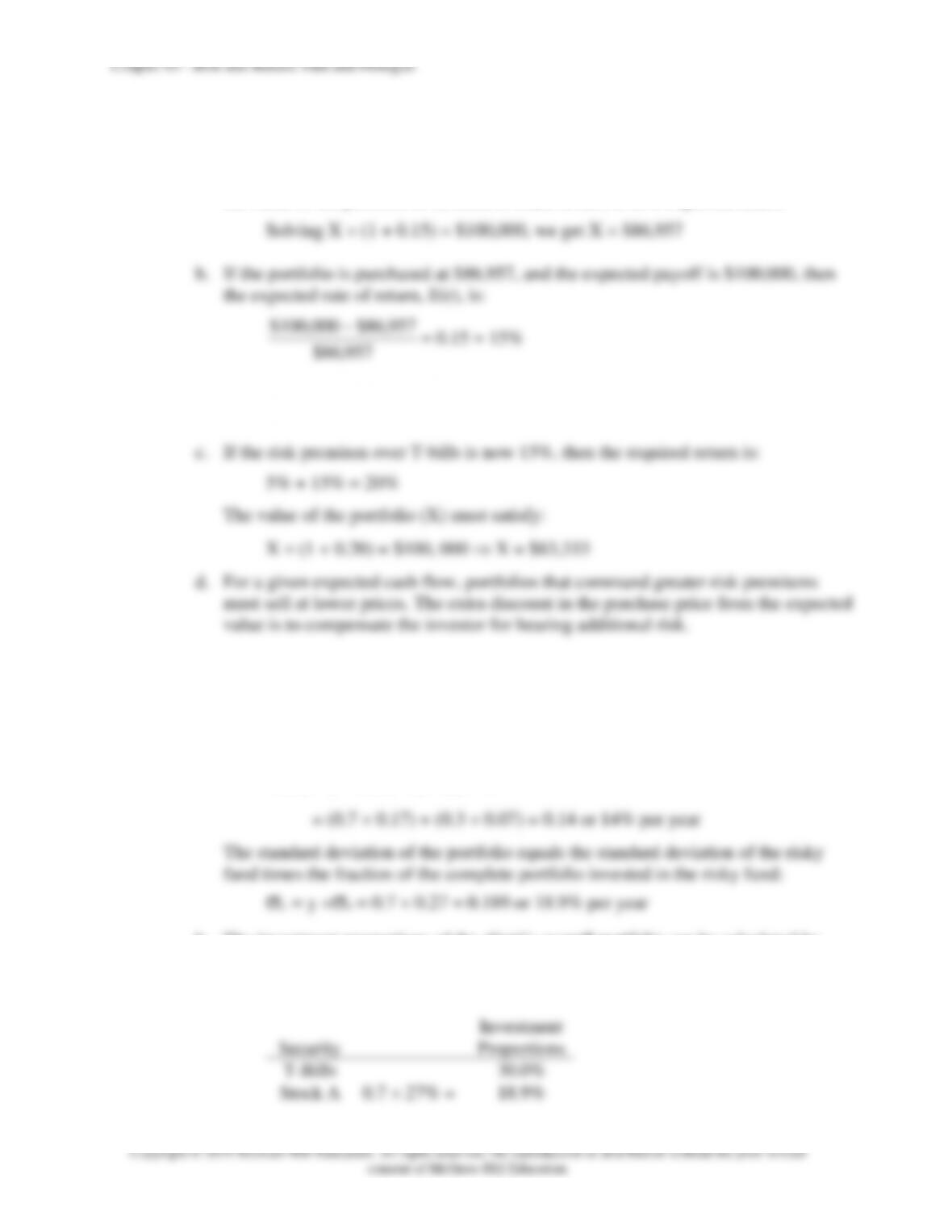
a. The expected cash flow is: (0.5 $50,000) + (0.5 $150,000) = $100,000
With a risk premium of 10%, the required rate of return is 15%. Therefore, if
the value of the portfolio is X, then, in order to earn a 15% expected return:
957,86$
The portfolio price is set to equate the expected return with the required rate of
return.
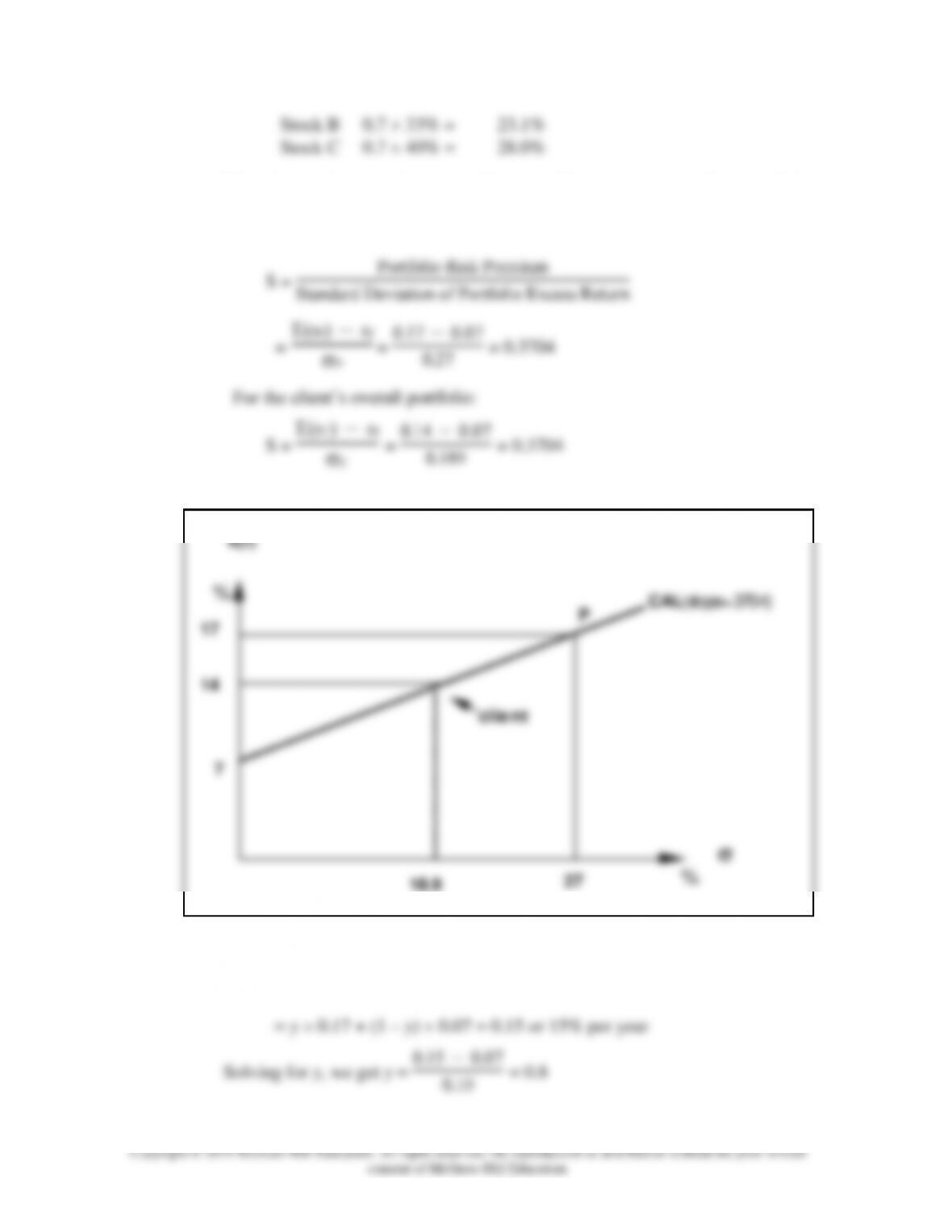
12. a. Allocating 70% of the capital in the risky portfolio P, and 30% in risk-free asset,
the client has an expected return on the complete portfolio calculated by adding
up the expected return of the risky proportion (y) and the expected return of the
proportion (1 – y) of the risk-free investment:
E(rC) = y E(rP) + (1 – y) rf
b. The investment proportions of the client’s overall portfolio can be calculated by
the proportion of risky portfolio in the complete portfolio times the proportion
allocated in each stock.
Chapter 05 – Risk and Return: Past and Prologue
Stock B
0.7 33% =
23.1%
Stock C
0.7 40% =
28.0%
c. We calculate the reward-to-variability ratio (Sharpe ratio) using Equation 5.14.
For the risky portfolio:
13.
a. E(rC) = y E(rP) + (1 – y) rf
Solving for y, we get y = 0.15 - 0.07
0.10 = 0.8
E(r)
7
27
14
17 P CAL ( slope=.3704)
%
%
18.9
clie nt
Chapter 05 – Risk and Return: Past and Prologue
Therefore, in order to achieve an expected rate of return of 15%, the client must
invest 80% of total funds in the risky portfolio and 20% in T-bills.
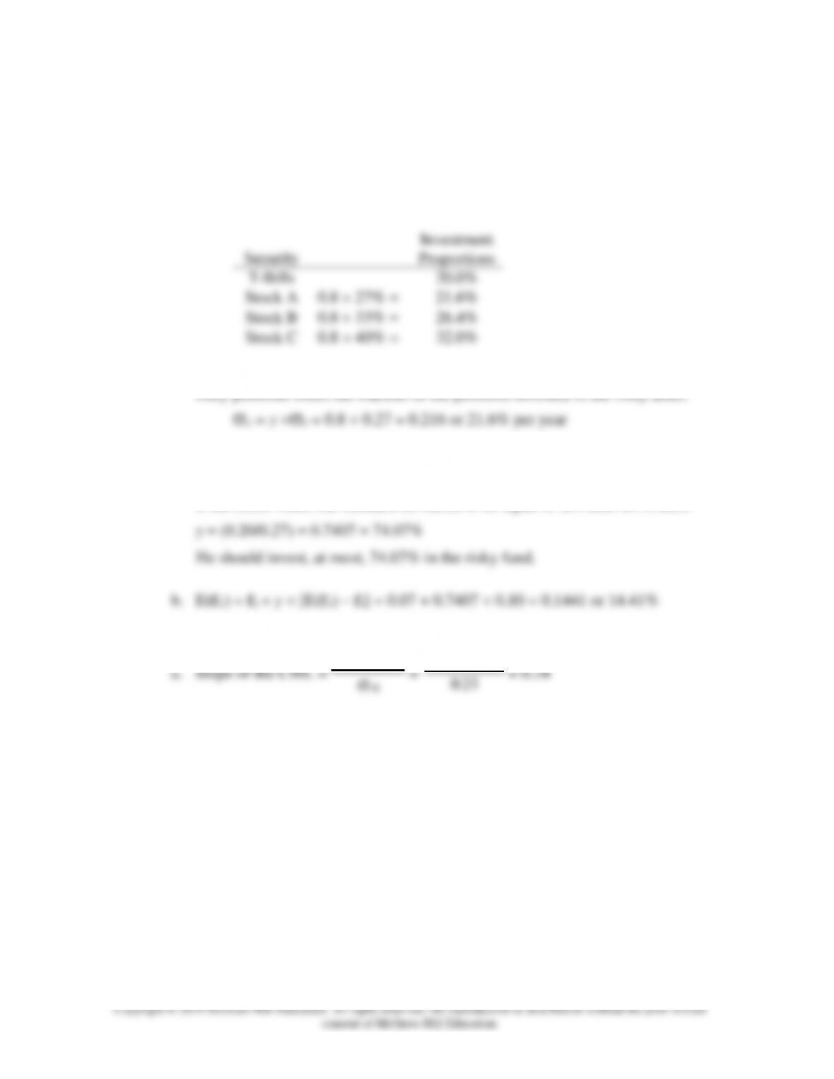
b. The investment proportions of the client’s overall portfolio can be calculated by
the proportion of risky asset in the whole portfolio times the proportion
allocated in each stock.
Chapter 05 – Risk and Return: Past and Prologue
Copyright © 2019 McGraw-Hill Education. All rights reserved. No reproduction or distribution without the prior written
consent of McGraw-Hill Education.
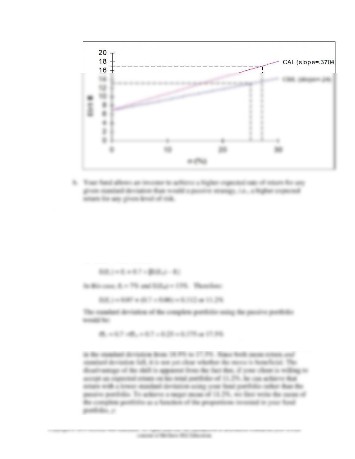
b. Your fund allows an investor to achieve a higher expected rate of return for any
given standard deviation than would a passive strategy, i.e., a higher expected
return for any given level of risk.
16.
a. With 70% of his money in your fund’s portfolio, the client has an expected rate
of return of 14% per year and a standard deviation of 18.9% per year. If he
shifts that money to the passive portfolio (which has an expected rate of return
of 13% and standard deviation of 25%), his overall expected return and standard
deviation would become:
Therefore, the shift entails a decline in the mean from 14% to 11.2% and a decline
Chapter 05 – Risk and Return: Past and Prologue
Copyright © 2019 McGraw-Hill Education. All rights reserved. No reproduction or distribution without the prior written
consent of McGraw-Hill Education.
E(rC) = 7% + y (17% – 7%) = 7% + 10% y
Because our target is E(rC) = 11.2%, the proportion that must be invested in your
fund is determined as follows:
11.2% = 7% + 10% y y = 11.2% - 7%
10% = 0.42
The standard deviation of the portfolio would be:
C = y 27% = 0.42 27% = 11.34%
Thus, by using your portfolio, the same 11.2% expected rate of return can be
achieved with a standard deviation of only 11.34% as opposed to the standard
deviation of 17.5% using the passive portfolio.
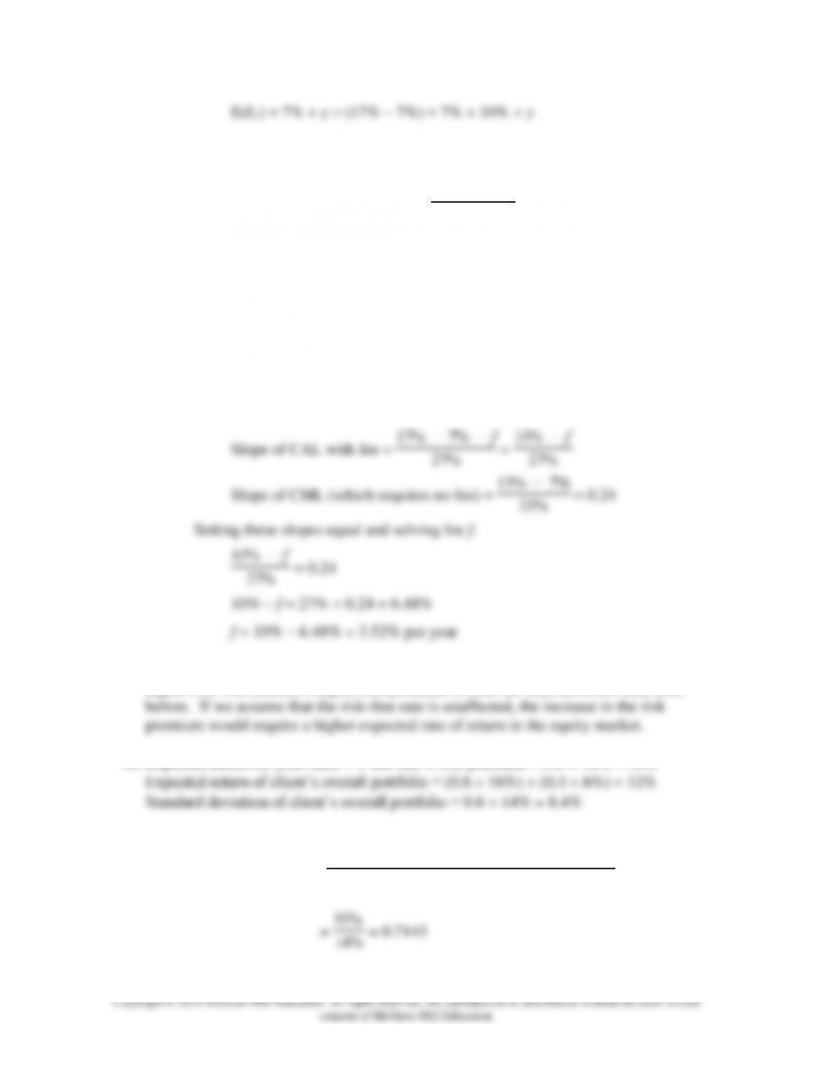
b. The fee would reduce the reward-to-variability ratio, i.e., the slope of the CAL.
Clients will be indifferent between your fund and the passive portfolio if the
slope of the after-fee CAL and the CML are equal. Let f denote the fee:
17. Assuming no change in tastes, that is, an unchanged risk aversion, investors perceiving
higher risk will demand a higher risk premium to hold the same portfolio they held
18. Expected return for your fund = T-bill rate + risk premium = 6% + 10% = 16%
19. Reward to volatility ratio = Portfolio Risk Premium
Standard Deviation of Portfolio Excess Return
20.
Excess Return (%)
21. For geometric real returns, we take the geometric average return and the real geometric
return data from Table 5.3 and then calculate the inflation in each time frame using the
equation: Inflation rate = (1 + Nominal rate)/(1 + Real rate) – 1.
Geometric Real Returns (%) – Large Stocks
Average
Inflation
Real Return
1926-2013
9.88
2.97
6.71
1926-1955
9.66
1.36
8.18
1956-1985
9.62
4.97
4.51
1986-2013
10.50
2.76
7.53
Risk Return Ratio – Large Stocks
Arithmetic Real
Return
Std Dev
Real Return to Risk
1926-2013
8.71
20.19
0.43
1926-1955
11.20
25.18
0.44
1956-1985
5.94
17.15
0.35
1986-2013
9.02
17.37
0.52
The VaR is not calculated.
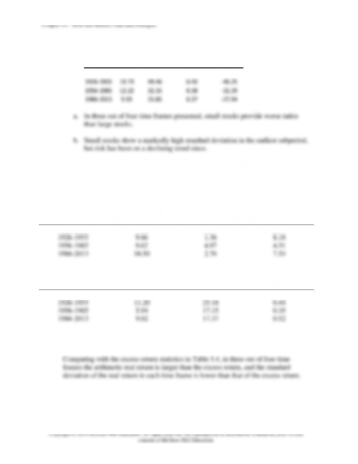
22.
Average Std Dev Sharpe Ratio 5% VaR
1926-2013 13.94 37.29 0.37 –36.96
1926-1955 19.73 49.46 0.40 –46.25
1956-1985 12.22 32.35 0.38 –32.39
1986-2013 9.59 25.85 0.37 –27.94
Chapter 05 – Risk and Return: Past and Prologue
Nominal Returns (%) – Small Stocks
Nominal Return
Std Dev
Return to Risk
1926-2013
17.48
36.73
0.48
1926-1955
20.82
49.10
0.42
1956-1985
18.06
31.88
0.57
1986-2013
13.30
25.20
0.53
Real Return (%) – Small Stocks
Arithmetic Real
Return
Std Dev
Return to Risk
1926-2013
14.14
36.08
0.39
1926-1955
19.04
48.34
0.39
1956-1985
12.80
30.85
0.42
1986-2013
10.32
24.89
0.41
The VaR is not calculated.
Comparing the nominal rate with the real rate of return, the real rates in all time frames
and their standard deviation are lower than those of the nominal returns.
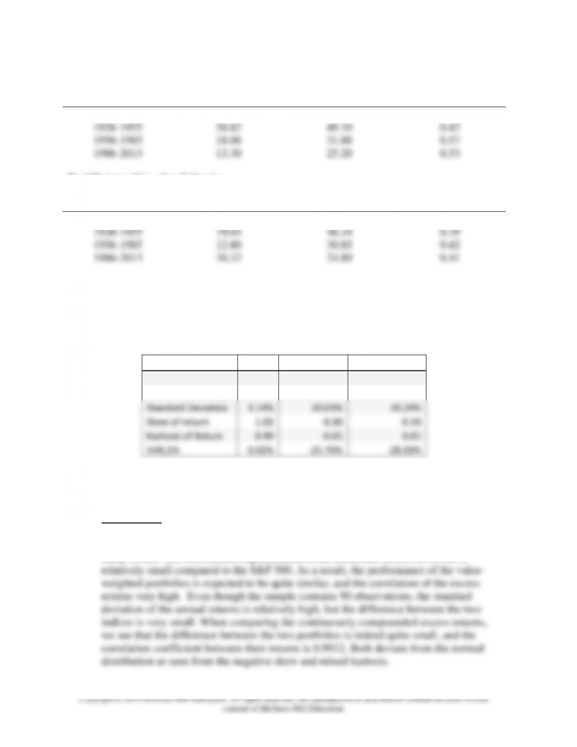
23. a.–e.
Results
T-Bill
S&P 500*
Market*
Arithmetic Average
3.43%
8.26%
8.48%
Geometric Average
3.38%
6.27%
6.43%
Standard Deviation
3.14%
20.03%
20.29%
Skew of return
1.02
-0.30
-0.33
Kurtosis of Return
0.99
-0.05
0.01
VAR,5%
0.02%
-25.76%
-28.03%
* Excess Returns
Comparison
The combined market index represents the Fama-French market factor (Mkt). It is
better diversified than the S&P 500 index since it contains approximately ten times as
many stocks. The total market capitalization of the additional stocks, however, is
Chapter 05 – Risk and Return: Past and Prologue
Copyright © 2019 McGraw-Hill Education. All rights reserved. No reproduction or distribution without the prior written
consent of McGraw-Hill Education.
As a result of all this, we expect the risk premium of the two portfolios to be similar, as
we find from the sample. It is worth noting that the excess return of both portfolios has
a small negative correlation with the risk-free rate. Since we expect the risk-free rate to
be highly correlated with the rate of inflation, this suggests that equities are not a
perfect hedge against inflation. More rigorous analysis of this point is important, but
beyond the scope of this question.
CFA 1
Answer: V(12/31/2016) = V(1/1/2010) (1 + g)7 = $100,000 (1.05)7 = $140,710.04
CFA 8
Chapter 05 – Risk and Return: Past and Prologue
Answer:
X2 = [0.2 (–0.20 – 0.20)2] + [0.5 (0.18 – 0.20)2] + [0.3 (0.50 – 0.20)2] = 0.0592
CFA 9
Answer:
E(r) = (0.9 0.20) + (0.1 0.10) = 0.19 or 19%
CFA 10
CFA 11