
Chapter 18 – Portfolio Performance Evaluation
CHAPTER EIGHTEEN
PORTFOLIO PERFORMANCE EVALUATION
CHAPTER OVERVIEW
This chapter presents various performance measures that are used for evaluation of portfolios.
The process of decomposing portfolio returns into the various components of the portfolio-
building process is presented. Performance measures of market timing, security selection and
adding securities to a diversified portfolio are introduced.
LEARNING OBJECTIVES
After studying this chapter, the student should be able to calculate various risk-adjusted return
measures, including Jensen’s alpha, the Sharpe and Treynor ratios, the M2 measure, and the
CHAPTER OUTLINE
1. Investment Clients, Service Providers, Objectives of Performance Evaluation
PPT 18-2 through PPT 18-18
Passive management consists of choosing a capital allocation between cash and the risky
portfolio and choosing the asset allocation within the risky portfolio. However, how passive the
management actually is varies from, “set it and forget it,” to changing allocations in according to
perceptions of risk to keep current with portfolio goals. Active management is a step beyond.
Active management involves forecasting future rates of return on either/both asset classes and
individual securities. Passive management, even if the portfolio is updated, is basically focused
on the level of risk of the portfolio in conjunction with the stated portfolio goals. Active
management is far more difficult. Risk levels are fairly stable but expected returns are not.
Successful forecasting of future prices and rates of return is very difficult in the highly
competitive markets we have. It requires either private information, or perhaps some better
analytical or instinctual method of analysis. A true market timer focuses on allocation between
the risky and riskless portfolios, although most actually change broad class allocations and
reallocate within the risky portfolio as well. It is a stretch to call a market timer a passive
investor, so there is a bit of ambiguity here.

Chapter 18 – Portfolio Performance Evaluation
Copyright © 2019 McGraw-Hill Education. All rights reserved. No reproduction or distribution without the prior written consent
of McGraw-Hill Education.
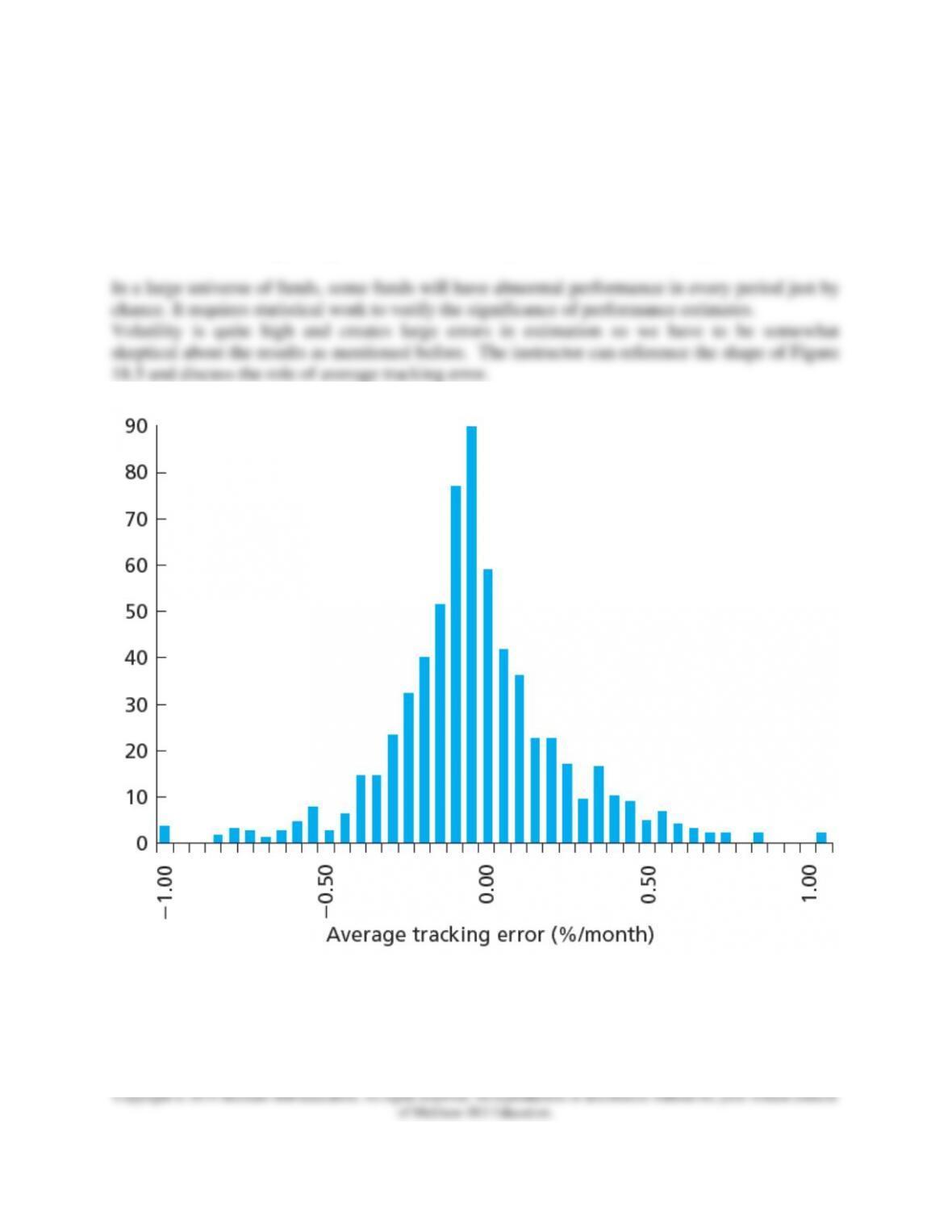
What is needed is a measure of abnormal performance. One can get more return in bull markets
by taking on more risk, this doesn’t mean the managers are adding value; can they generate good
returns consistently through time across different market cycles? It takes measures that
incorporate risk and it requires statistical work to make us believe the results are not just due to
chance.
How can managers generate abnormal performance? There are several means:
• Successful across asset allocations (time the market)
• Superior allocation within each asset class (weight sectors)
o Sectors or industries
o Overweight better performing sectors, underweight poorer performers
• Individual security selection (pick stocks)
o Pick the right stocks, those with performance better than expected
The most valuable activity and the toughest to do successfully is time the market.
Obtaining an accurate estimate of risk-adjusted performance for a portfolio manager is difficult
for several reasons. First, in order to measure abnormal performance one needs an accurate
model of normal performance. Is a single index model an adequate measure of expected
performance or should a multi-index model be used? Second, most of the sound measures of
risk-adjusted returns require stability for the portfolio. Most portfolios are actively managed and
the stability assumptions are not met. Third, in competitive markets with significant volatility,
identifying the actual level of abnormal performance that is likely to occur is very difficult. The
probability of a Type 2 error is quite high.
Basic performance measurement compares portfolio performance to some benchmark portfolio.
The comparison to the benchmark is only appropriate if the risk is the same. Comparison groups
are very popular within the industry. It is the simplest method and involves comparing
performance of funds with similar objectives. The market model or index model approaches are
theoretically superior because they explicitly adjust for different levels of systematic risk.
The Sharpe Measure is also widely accepted in industry. This measure indicates the slope of the
CAL and it is based on the portfolio risk premium and the total risk of the portfolio as measured
by standard deviation.
p
fp
σ
rr
Ratios Sharpe −
=

Chapter 18 – Portfolio Performance Evaluation
The Treynor measure also calculates the excess return to variability ratio but it uses the portfolio
beta as the risk measure. The Sharpe and the Treynor measures should result in similar rankings
for most widely diversified portfolios. With portfolios that are widely diversified, most of the
risk will be systematic.
One may want to compare the reward to risk ratios where risk is measured as solely systematic
risk.This measure asks the question, “How much excess return does one get for the level of
risk?” In a well diversified portfolio systematic risk will be the only remaining risk. This
measure might still be useful if we are analyzing a non-diversified portfolio such as a sector fund
that is held in conjunction with other funds that in total are diversified. This is an important
point to stress to the students.
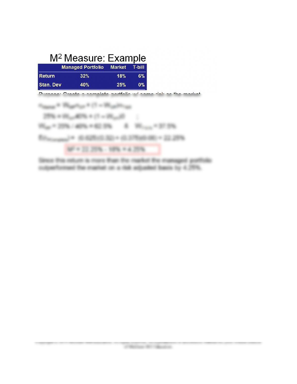
The M2 measure is a variation of the Sharpe Ratio that is easier to interpret. The concept of the
Sharpe is easy to interpret but the Sharpe number is not. It was developed by Modigliani and
Modigliani; hence M2. One uses M2 to compare the performance of a managed portfolio (MP)
with a market index. The M2 measure creates a hypothetical complete portfolio that is composed
of T-bills and the MP that has the same standard deviation as the market index. This allows
comparing the portfolio return directly with the level of return of the market.
p
fp rr
Ratios Treynor
−
=
*
*
2()
M M P M
P
M
P P M P
PP
M
M M M M
M
M R R S S
where
R wR R S
R
RS
= − = −
= = =
==
Chapter 18 – Portfolio Performance Evaluation
Copyright © 2019 McGraw-Hill Education. All rights reserved. No reproduction or distribution without the prior written consent
of McGraw-Hill Education.
When evaluating a portfolio to be mixed with a position in the passive benchmark portfolio one
must draw on insights of the Treynor-Black (TB) Model (See Chapter 6 for this model.)
If you are a fund manager you may try to analyze several companies. If a manager has the ability
to find undervalued stocks, what strategy should a portfolio manager use in investing in those
stocks? The percentage of funds allocated to undervalued stocks depends, in part, on the ability
of the manager. If a manager has perfect foresight, theoretically all funds should be placed in the
most undervalued stocks. If the manager has substantial funds however, buying pressure could
make that impossible. The risk of such a strategy would be extreme in any case. Most portfolio
managers would not have perfect ability in identifying undervalued securities. For most
managers, the process involves some passive investment in stocks in addition to acquiring the
undervalued stocks. The Treynor-Black Model is used to combine an actively managed portfolio
with a passively managed portfolio. To determine the optimal allocations the portfolio managers
must be able to forecast expected returns and risk for both the actively managed and passively
managed portfolios. The relevant measure of risk for the actively managed portfolio is its ratio
of alpha to nonsystematic risk.

Chapter 18 – Portfolio Performance Evaluation
Using a reward-to-risk measure that is similar to the Sharpe Measure, the optimal combination of
active and passive portfolios can be determined. The idea is to choose the portfolio, which when
combined with the passive benchmark, generates an efficient frontier with the best return per unit
of risk as measured by the standard deviation. This is found by combining the Sharpe ratio of
the benchmark M with the information ratio of portfolio P:
Summary of measures and usage
Performance
Measure Definition Application
Sharpe p
R/
as the
When choosing
among portfolios
competing
optimal risky portfolio
Treynor Rp/
When ranking many
portfolios that will be
mixed to form the
optimal risky portfolio
Information
ratio p
/ e
When evaluating a
portfolio to be mixed
with a position in the
passive benchmark
portfolio
→
This edition of the text goes much further in explaining alpha and its relationship to other
performance measures.
= Correlation between RP & RM
A positive alpha does not guarantee a higher Sharpe than the benchmark because SM(r-1) < 0.
Thus a positive alpha is a necessary but not a sufficient condition for net performance
improvement.
The alpha must be large enough to offset increase in residual risk from moving away from the
diversified optimum. Take note though that this conclusion about alpha changes if one can use
short sales and hedge out the risks.
Alpha and the Treynor measure
A positive alpha does not guarantee a higher Treynor ranking because one must know the beta as
well. Alpha and the Information Ratio:
P
P
MMP )1(SSS
+−=−
P
P
MP TT
=−
P
e
P
σ
α
Ratio nInformatio =

Chapter 18 – Portfolio Performance Evaluation
A positive alpha does not guarantee a higher square of the information ratio because a higher
alpha may come with higher residual risk.
Alpha Capture & Transport
If an analyst finds an undervalued security and invests in it, market moves may still wipe out any
gains. Remember this is called fundamental risk. However, one can hedge out market risk via
shorting a stock index or stock index futures to establish a market neutral position. Recall that
ETFs can be shorted.
This should eliminate any systematic risk and leave the investor with the stock’s positive alpha.
The process to establish a zero beta or market neutral position is called alpha capture or alpha
transport.
To hedge out systematic risk, short sell βP dollars of the index for every dollar invested in the
portfolio, investing the proceeds in T-bills. The excess return on this zero beta position is:
(the excess return per $ invested in P)
(the excess return on the β dollars sold in M)
(the excess returns on the T-bills is always zero)
The Sharpe ratio for Z, SZ, simplifies to the information ratio because ρ = 0 by construction
because with a zero beta, the correlation between Z and M = 0. Note that one could write alpha
as alpha p or alpha z.
When short positions and leverage are allowed a significant non-zero alpha is a sufficient
condition for an improvement in the Sharpe and information ratio. Because this hedge portfolio
establishes a zero beta portfolio, the Treynor measure is undefined. Note that the evidence
indicates that it is difficult to find positive alphas, although it may be easier to find negative
alphas.
Evidence indicates one should use a multi-index model such as the Fama-French model (FF)
(See Chapter 7) to establish the expected return:
This allows an estimation of alpha:
ptPMtPPt eαRβR++=
ptPMtPZ eαRβR++=
MtPRβ−
0
ptPZ eαR+=
P
ZαR=
P
P
Z
P
P
MMZ S or )1(SSS
=
+−=−
ptPHMLtHMLSMBtSMBMtPPt eαrβrβRβR++++=
P
HMLt
HML
SMBt
SMB
Mt
P
Pt αrβrβRβR+++=

Chapter 18 – Portfolio Performance Evaluation
Copyright © 2019 McGraw-Hill Education. All rights reserved. No reproduction or distribution without the prior written consent
of McGraw-Hill Education.
If the multi-index model is a better estimator of expected returns then alphas deemed significant
from a single index model are suspect. Evidence indicates that the indices such as the S&P500
have positive alphas when calculated against the FF model, even when a fourth momentum
factor is added. This probably tells us we still don’t have the proper model of expected returns
so all performance evaluation should be viewed skeptically.
The assumptions of stability that underlie the measures of abnormal performance limit their
effectiveness. Actively managed portfolios are, by their nature, not stable. The beta of the
portfolio may be changing substantially over the measurement period. Use of the average beta
for the period could lead to errors in assessing abnormal performance.
2. Style Analysis
PPT 18-19 through PPT 18-22
In recent years style analysis has become popular with the investment industry. The initial work
in style analysis was conducted by Nobel Prize winner Bill Sharpe. A 1992 study of mutual fund
performance found that 91.5% of variation in return could be explained by the funds’ allocations
to bills, bonds and stocks. Style analysis attempts to explain percentage returns by allocation to
style. Style analysis has become popular with the industry.
3. Morningstar’s Risk-Adjusted Rating
PPT 18-23 through PPT 18-24
The Morning Star Rating System has also become very popular with the investment community.
The risk adjusted returns they report are very highly correlated with the Sharpe Ratio. The Star
System ranks funds within peer groups based on percentiles as follows:
The catch is that star ratings are based on historical performance and don’t necessarily predict
future performance.
Chapter 18 – Portfolio Performance Evaluation
4. Risk Adjustment with Changing Portfolio Composition
PPT 18-25 through PPT 18-26
Performance measures assume a fund maintains a constant level of risk. This assumption is
violated for most funds and is particularly problematic for funds that engage in active asset
allocation. To see how this affects performance the text constructs a simple example that
students readily grasp and is reproduced here:
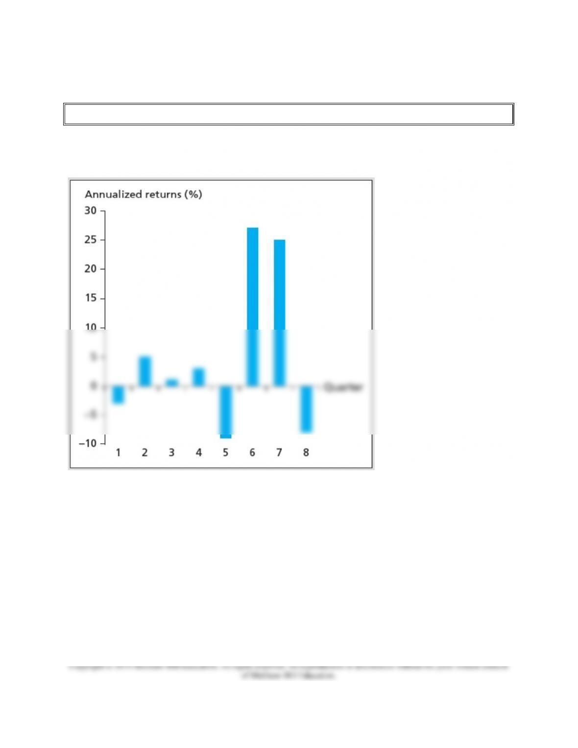
Suppose the Sharpe of the benchmark M = 0.4. We want to know if the active portfolio returns
depicted in the graph generated a superior Sharpe ratio. The fund used a low risk strategy for the
first four quarters and then switched to a high risk strategy for the final four quarters and
generated the following set of excess returns:
First 4 qtrs excess returns are -3%, 5%, 1% and 3%, consistent with the predicted mean and SD
2nd 4 qtrs excess returns are -9%, 27% , 25% and -8%, also consistent with predictions for the
higher volatility period.
Chapter 18 – Portfolio Performance Evaluation
In both years the fund outperformed M which had a Sharpe of 0.4. However if one calculates the
fund’s Sharpe over all 8 quarters one finds an average excess return of 5.125% and a standard
deviation of 13.8% for an Overall Sharpe ratio = 0.37. Switching strategies in the middle creates
the appearance of volatility. Note this violates the assumption of stationary risk. If one didn’t
know about the strategy change one would incorrectly state that the fund underperformed M.
5. Market Timing
Chapter 18 – Portfolio Performance Evaluation
PPT 18-26 through PPT 18-31
If a portfolio manager could time general movements in the market, the performance would be
similar to a call option. When market returns are lower than money market instruments, the
manager would switch out of equities and into money markets. When stock returns will be
higher than money market instruments, all of the funds would be invested in stock. The result
would be higher returns and a smaller standard deviation. A graphical display of perfect market
timing is displayed in the PPT. With less than perfect timing ability, the problem of identifying a
superior market timer becomes a much more difficult task. A long horizon is needed to measure
the ability to time the market to ensure that the manager truly has superior ability to time. We
have not seen a large number of bull and bear markets in recent years. This reduces the accuracy
of testing a manager’s ability to call turns. If the manager of a portfolio can time the market, that
manager would increase the beta on the portfolio when the market is expected to rise. When the
market experiences lower returns or losses, the manager reduces the beta of the portfolio.
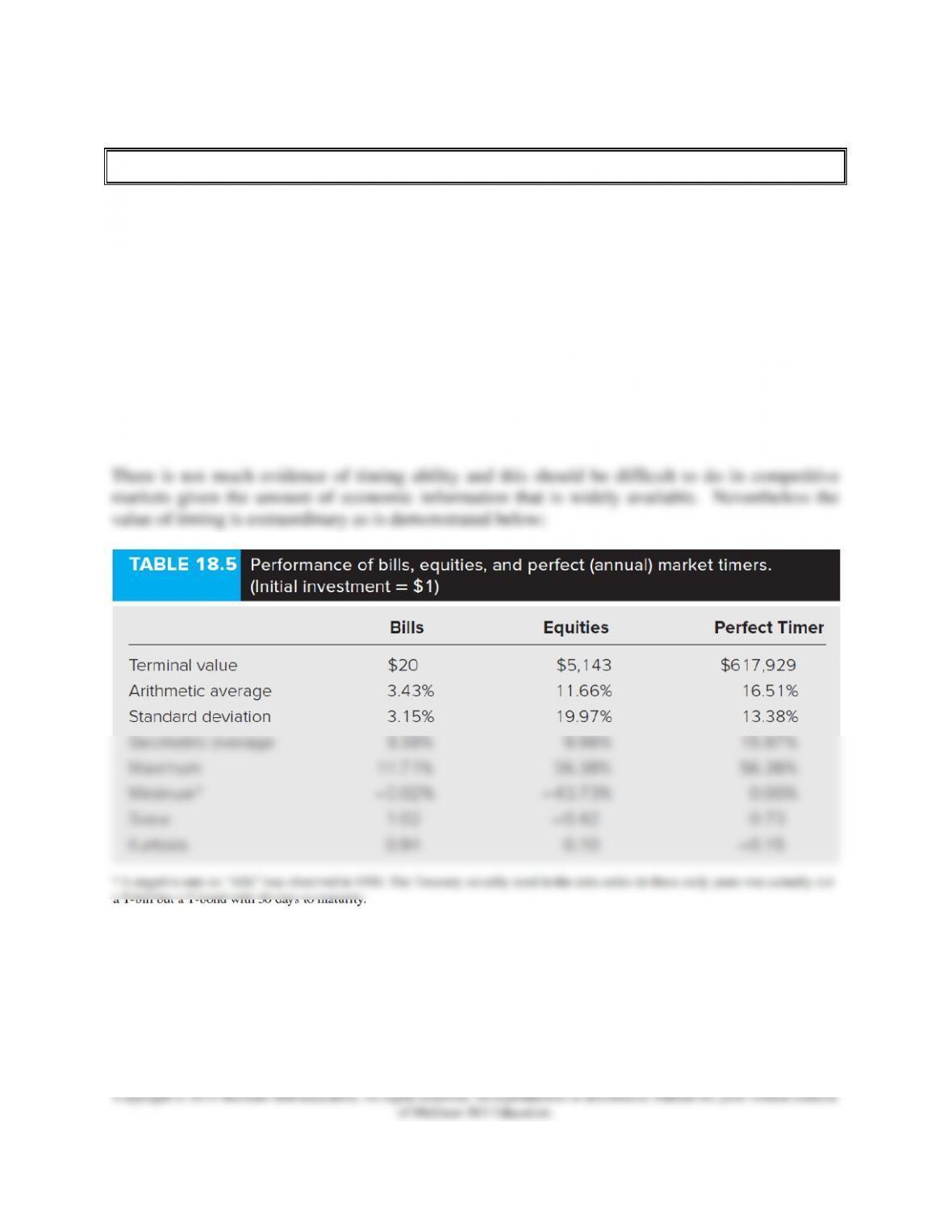
The timer doesn’t have to perfectly forecast the cash or the stock market, he or she just has to
know which one will do better. The time period is 82 years so part of the size of the numbers is
the long time period for compounding. As stated above, there isn’t much evidence of timing
ability but one can understand the lure of it with the size of gains that are possible.
6. Performance Attribution Procedures
Chapter 18 – Portfolio Performance Evaluation
PPT 18-32 through PPT 18-36
Decomposing overall performance into components allows the analyst to determine what aspects
of portfolio choices contributed to good or bad performance.
Major performance determinants include the broad asset allocation among types of securities,
industry weighting in equity portfolio, security choice, and the timing of purchases and sales.
We would like to be able to ascertain the effects of these choices on portfolio performance.
The second step is to calculate the contribution to performance of both sector and security
selection. The next step is to calculate the contribution of the equity sector allocation to total
performance. Finally the security selection component can be inferred by subtracting the sector
allocation return from the total equity extra return. The analysis concludes with a summary of
the performance differences into appropriate categories. Table 18.6 offers a useful example in
the PPT.
Excel Applications
Two Excel applications can be used to enhance the students’ understanding of the material
covered in this chapter. The first application allows the students to perform attribution analysis.
The second application calculates the performance measures presented in this chapter. It allows
students to compare the measures and rankings.