Unlock document.
This document is partially blurred.
Unlock all pages and 1 million more documents.
Get Access
Chapter 16 - Option Valuation
Copyright © 2019 McGraw-Hill Education. All rights reserved. No reproduction or distribution without the prior written consent
of McGraw-Hill Education.
CHAPTER SIXTEEN
OPTION VALUATION
CHAPTER OVERVIEW
This chapter discusses factors affecting the value of an option and presents analytical and
spreadsheet models of option pricing. Put call parity is introduced, manipulating hedge ratios
and portfolio insurance techniques are also presented.
LEARNING OBJECTIVES
After studying this chapter, the student should be able to identify the characteristics that
determine an option’s value and should understand how different values for these variables affect
CHAPTER OUTLINE
1. Option Valuation: Introduction
PPT 16-2 through PPT 16-5
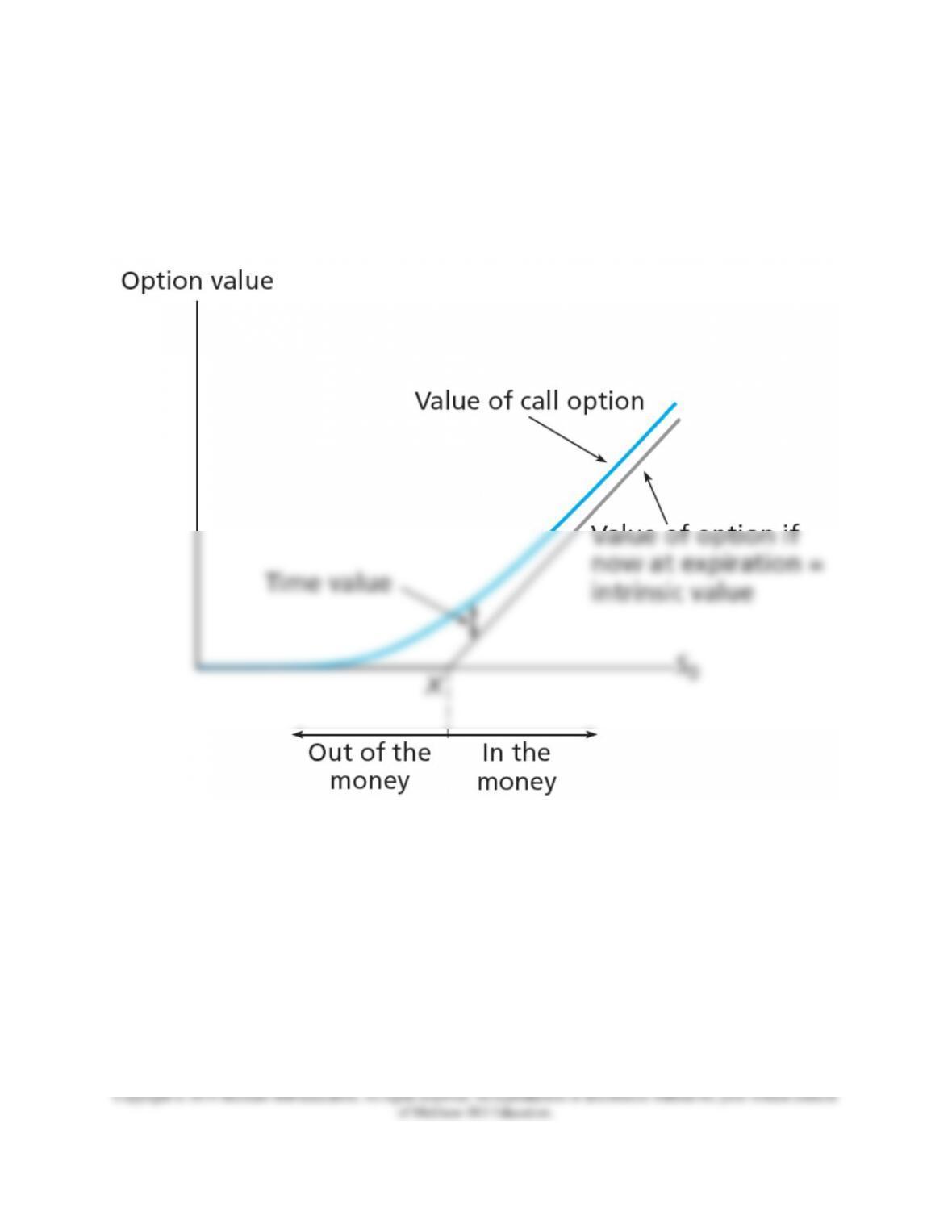
When describing options, intrinsic value refers to the value if the option were immediately
exercised. Exercise value was introduced in Chapter 15 in the Instructor’s Manual because this
helped students understand basic option strategy payoffs. A review is provided below:
Basic boundaries revisited
Ct ≥ 0, Why?
Ct ≥ St – X, Why?
Thus Ct ≥ Max (0, St – X)
where:
Ct = Price paid for a call option at time t. t = 0 is today,
T = Immediately before the option's expiration.
Pt = Price paid for a put option at time t.
St = Stock price at time t.
X = Exercise or Strike Price (X or E)
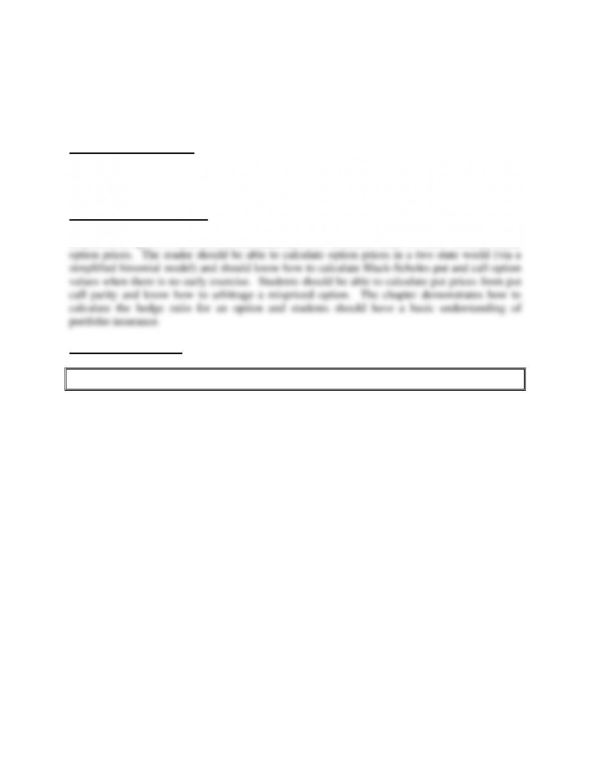
A tighter boundary can be developed by considering two different portfolios:
Portfolio 1: Long position in stock at S0
Portfolio 2: Buy 1 at the money call option (C0) and buy a T-bill with a face value = X.
Chapter 16 - Option Valuation
Copyright © 2019 McGraw-Hill Education. All rights reserved. No reproduction or distribution without the prior written consent
of McGraw-Hill Education.
From here we can present the value of a call option at expiration and prior to expiration as
follows:
Chapter 16 - Option Valuation
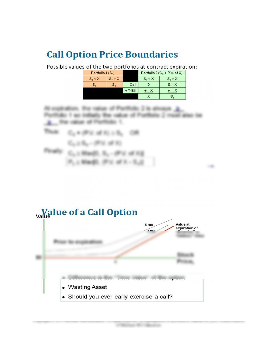
The difference between the value prior to expiration (curvilinear values) and the exercise or
intrinsic value Max(0,S-X) is the time value of the call. The option is a ‘wasting asset’ that loses
value as expiration approaches. This is the same for put and this is referred to as a – Theta
position. (Writing an option will be a + Theta position.) Going long or buying an option is a play
that the price will move enough before you run out of time value.
The time value of a call incorporates the probability that S will be in the money at period T given
S0, time to T, s2stock, X, and the level of interest rates. The benefit of time value is the chance
that the option will wind up further in the money. Of course, it might not wind up further in the
money, but remember the asymmetric outcome; if it finishes out of the money one just doesn’t
use it.
Note that you should never early exercise the call option since that would be sacrificing the
difference between the option value and the intrinsic value (the curvilinear value – intrinsic
value). Actually you might early exercise if the stock paid a large enough dividend so that you
could receive the dividend. If the dividend is greater than the time value on the call, you would
want to early exercise right before the stock went ex-dividend.
Chapter 16 - Option Valuation
2. Binomial Option Pricing
PPT 16-6 through PPT 16-12
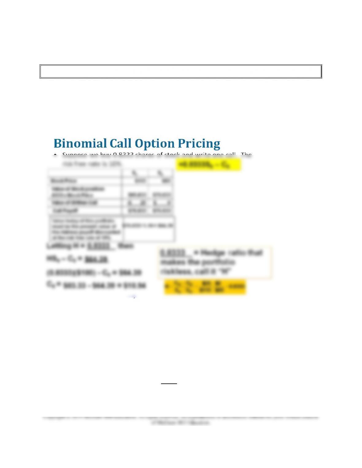
A binomial pricing example is developed. For example, assume the stock is currently priced at
$100 and will have a value of either $115or $85 at the end of the period. A call that has an
exercise price of $90 will be worth $0 or $25 at the end of the period. The problem with trying
to value the call is that one doesn’t know what discount rate to use due to the option risk. This is
the problem that stumped Fischer Black, Myron Scholes and others before the development of
the idea of the riskless hedge.
If one buys H = 0.8333 shares of stock per call written the resulting position will be riskless.
The strategy’s payoff is $70.833 in either state of the economy. Its present value can be found
by discounting $70.833 at the risk free rate of 10% for one period, obtaining $64.39. The current
value of this portfolio HS0 – C0 = $64.39. S0 is known and is equal to $100, so it is trivial to
solve for C0 = $18.94. H is the hedge ratio in the binomial framework and its calculation is
provided above. Conceptually H is roughly analogous to ∆C/∆S.
The call value is > the exercise value of the call option.
Call value today = $18.94
Call intrinsic value or exercise value = 10.00 = ($100 - $90)
Time value of the call = $ 8.94
Chapter 16 - Option Valuation
While the two-state approach is simplistic, the approach is easily generalized. Expansion of the
two-state approach shows how the probability distributions will approach the familiar bell
shaped curve as the number sub-periods increases.
3. Black-Scholes Option Valuation
PPT 16-13 through PPT 16-24
The Black-Scholes (BS) option pricing model is:
C0 = Current call option value. X (or E) = Exercise Price
S0 = Current stock price, δ = Annual dividend yield on the stock
e = 2.71828, the base of the natural log
r = Risk-free interest rate (annualize with continuous compounding the return on a T-bill with
the same maturity as the option: To convert a regular return to a continuously compounded
return take Ln (1 + return)
T = Time until expiration (not a point in time) in years,
σ = Annual standard deviation of continuously compounded stock returns
N(d) = probability that a random draw from a normal distribution will be less than d.
Including the annual dividend yield is an approximation of a discrete payment, (also technically
the dividend can’t be stochastic). It assumes no early exercise due to the dividend.
The exercise value of the call is S0 – X,
However if the call will not be exercised early the value today is S0 – the present value of X so
this boundary tightens up to S0 – X(e-rT). The cash dividend yield term δ reflects that a dividend
will reduce the stock price thus hurting the value of the call as is in the following: S0e-T – X(e-rT)
The term d1 comes from our assumptions about how stock prices move in continuous trading:
• E(r) = (r + σ2/2)T when returns are lognormally distributed
1
• Ln (S0 / X) measures the continuous return needed for the stock to finish in the money
• Roughly speaking the d1 numerator is a measure of the return needed to finish in the
money, the denominator measures this relative to the standard deviation of the returns.
N(d) is cumulative normal probability. It can be calculated in Excel using the
NORMSDIST function or one can look up the probability in a normal density table.
1
The non continuously compounded returns are lognormally distributed. When we convert them to continuously compounded
returns rcont = Ln(1+rsimple), the rcont are normally distributed. If you have simple stock return series for monthly data or shorter,
you don’t need to do the conversion to continuous compounding because they will give you approximately the same numbers
(albeit this is a rule of thumb heuristic).
Tσ
Chapter 16 - Option Valuation
Thus the N(d) terms can be thought of as a measure of the probability of how far in the money
the stock price is likely to be at expiration.
A spreadsheet model of the BS formula is also included below:
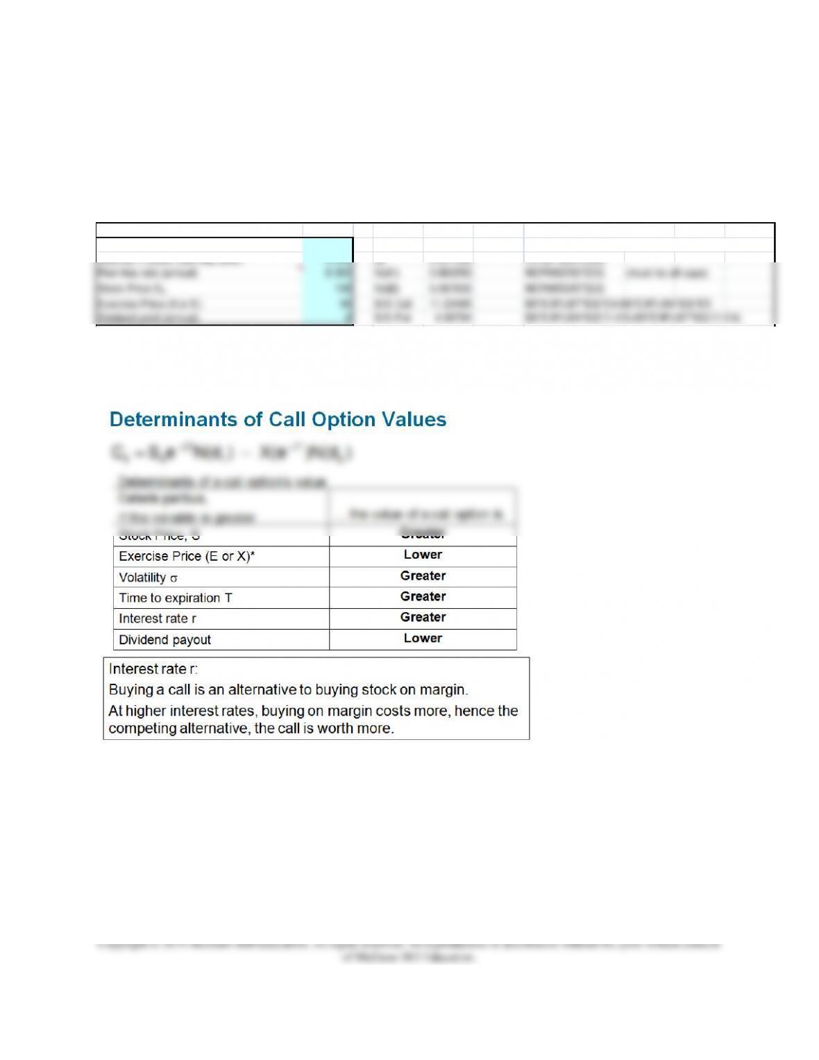
Once the model has been developed it is worthwhile to go over the comparative statics of the
model:
Black-Scholes model with dividends Outputs Formula for Output in Column E
Annual Standard deviation of stock's returns 0.400 d1 0.421466 (LN(B5/B6)+(B4-B7+0.5*B2^2)*B3)/(B2*SQRT(B3))
Maturity in years (365 day year) 0.250 d2 0.221466 E2-B2*SQRT(B3)
Dividend yield (annual) 0 B/S Put 4.99794 B6*EXP(-B4*B3)*(1-E5)-B5*EXP(-B7*B3)*(1-E4)
Chapter 16 - Option Valuation
The only variables difficult for students to understand are the volatility and the interest rate.
Higher volatility or stock risk increases a call option’s price because the greater volatility
increases the probability that the option will wind up (deeper) in the money by expiration.
Higher volatility also indicates that the stock may not wind up in the money even if it currently
is. However, due to the asymmetric nature of options (one don’t use them if they don’t help)
volatility increases value. An extreme example might help here. Suppose one has a stock priced
at $30 and a call option on the stock with an exercise price of $50. Would one pay more for the
option if the stock’s standard deviation was 0.0001% per year of if the stock’s standard deviation
was 30% per year? In the former case the option is highly unlikely to ever have exercise value,
but not in the latter case. The interest rate variable may require more explanation as per the note
above. A greater time to expiry increases the option premium simply because one has the option
for a longer time. Because X is the price one must pay to exercise, a higher X results in a lower
call value. Likewise since the option is the right to buy at the fixed value X, a higher S results in
a higher call value. Note that X would change if a stock split or stock dividend occurred, but not
otherwise. For instance, in a 2 for 1 stock split the exercise price would be halved. No
adjustment is made to X for a cash dividend.
This model is an approximation only for an American put because of the possibility of early
exercise of an American Put. This means that it can give you wrong estimates of value for deep
in the money American puts.
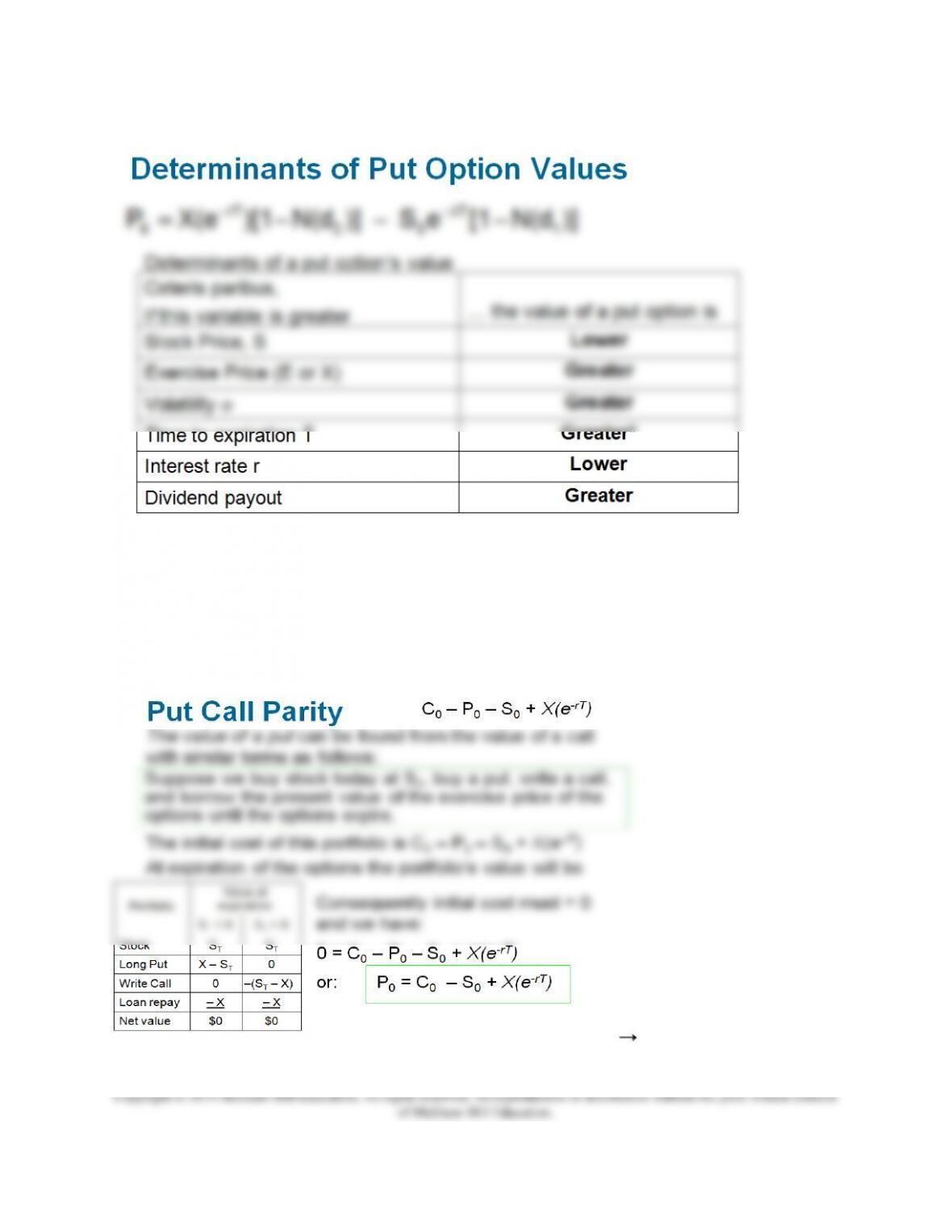
Determinants of put option values are as follows:
Chapter 16 - Option Valuation
The interest rate variable probably requires some explanation. A higher interest rate lowers the
PV of X, thereby lowering the put value. In concept, the most you can get from a put is X, and
the lower the PV of X the lower the value of the put. Buying a put is conceptually equivalent to
shorting the stock and investing the proceeds in X. With a higher interest rate the bond one is
buying is worth less.
Put call parity can be illustrated with a profit table from a replicating portfolio as follows:
Chapter 16 - Option Valuation
This combination will always result in a zero payoff at expiration so its initial cost must be zero
as well. This establishes the time zero value of 0 = C0-P0-S0 + X(e-rT). Knowing the call value
and the other variables one can find the implied put value. Using the BS model for puts will give
the same value. Both are correct only for European puts if there is a possibility of early exercise.
4. Using the Black-Scholes Formula
PPT 16-25 through PPT 16-33
The BS hedge ratio H can be found for a call option on a non-dividend paying stock as:
This means that the call option’s value will move by approximately N(d1) dollars when the
stock’s price moves one dollar. H approaches +1 as a call moves into the money. As a call
moves out of the money H approaches 0. One can use this concept to exploit a call price that
appears to be mispriced according to the Black-Scholes model as is illustrated in the PPT.
The BS hedge ratio H can be found for a put option on a non-dividend paying stock as:
H approaches -1 as a put moves into the money. As a put moves out of the money H approaches
0. The sensitivity of a position’s value to a change in stock price is sometimes called the
position’s Delta.
If the position is not affected by a change in stock price the position has a delta of zero and is
said to be delta neutral.
• If a position increases in value when stock price increases (and vice versa) it is positive
delta.
• If a position increases in value when stock price decreases (and vice versa) it is negative
delta.
The position delta can be strategically manipulated as market conditions change and this idea is
the basis for portfolio insurance strategies accomplished through dynamic hedging. The basic
concept of portfolio insurance involves the purchase of protective puts. Purchase of protective
puts is a relatively easy concept but there are some limitations to the implementation of portfolio
insurance. Since indexes are commonly used for the puts, tracking errors are possible. The
maturities of the puts are often too short.
Even if the portfolio of stocks remains constant, the deltas change as the stock prices change.
The concept of the delta changing as prices change is shown graphically.
S
0
S
0
Chapter 16 - Option Valuation
Option elasticity with respect to stock price is high due to option leverage; a 5%-10% change in
option price per 1% change in stock price would not be atypical. Further out of the money
options have greater elasticity, deep out options may have elasticities of 25% or more. Deep in
the money options may have elasticities as low as 2-3% but they have to be deep in.
The B-S model has been heavily tested with the general conclusion that the model generates
option values that are very close to actual market prices. However, there are some problems with
the model
• Stocks with high dividend payouts may lead to early exercise of a call option. The
model does not consider early exercise so B-S prices may be inaccurate in these cases.
One way to handle early exercise is to assume the call will be exercised on the day before
the stock goes ex-dividend. This is an inexact measure because the probability of early
exercise is not 100% but it may improve the call value estimate.
• Options on the same stock with the same expiration date should all have the same implied
volatility & they don’t. Implied volatility is higher for calls (puts) with low (high)
exercise prices. This may mean investors believe there is a greater probability of a market
crash than is implied by the continuous price movements assumed by the B-S model.
Excel Applications
Chapter 16 has an Excel spreadsheet that is available on the web site. The model allows the
students to find the value of puts and calls using Black-Scholes and also allows them to
investigate the factors that influence put and call values.


