
Solutions to Questions – Chapter 23
Real Estate
Investment
Funds:
S
tructure
,
P
erformance
,
Benchmarking,
and
Attribution
Analysis
Question 23-1
What are the primary differences between an open-end and closed-end fund? Why would an investor
choose to invest in one or the other?
Question 23-2
What is the difference between a time-weighted return and an internal rate of return? When reporting
historical investment performance to investors in a core fund, which return would be more likely to be
reported? What return would likely be used for an opportunity fund?
Question 23-3
Which type of fund, core or opportunistic, would you expect to have higher returns? Why? Which
would be expected to have greater volatility in returns? Why?
Question 23-4
What is meant by a target return? How does it relate to an investment benchmark?

Question 23-5
When comparing investment funds, what is the difference between committed capital and invested
capital? Why may this matter for investors?
Question 23-6
When evaluating investment funds, what is meant by performance at the “fund level” and at the
“property level”? What would generally cause a difference between the two? What is this difference
called?
Question 23-7
When thinking about the extent of discretion that fund managers have when making property
acquisitions, under which fund structures would a manager tend to have the greatest discretion? Under
which structures would they tend to have the least discretion? Why?
Question 23-8
When reporting property values to investors in funds, which fund types would generally require more
frequent appraisals than others? Why?
Question 23-9
What are the objectives of performing an attribution analysis? How could fund managers be evaluated
by using an attribution analysis?
Question 23-10
When evaluating fund performance, what is meant by “style drift”? How might style drift impact
investment returns and volatility?
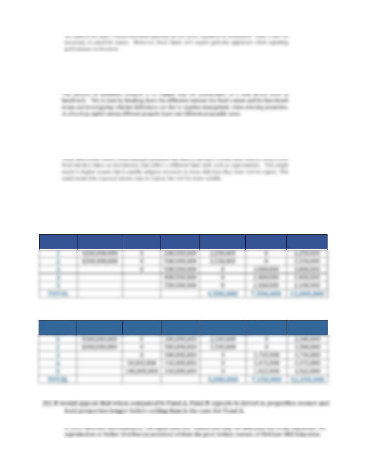
PROBLEM 23-1
FUND A: Capital Commitment $500,000,000
Year
Capital
Contribution
Capital
Returned
Capital
Invested
Fee on
Commitment
Fee on
Investment
Total Fee
1
$200,000,000
0
200,000,000
2,250,000
0
2,250,000
2
$300,000,000
0
500,000,000
2,250,000
0
2,250,000
3
0
500,000,000
0
3,000,000
3,000,000
4
400,000,000
0
2,400,000
2,400,000
5
350,000,000
0
2,100,000
2,100,000
TOTAL
4,500,000
7,500,000
12,000,000
FUND B: Capital Commitment $500,000,000
Year
Capital
Contribution
Capital
Returned
Capital
Invested
Fee on
Commitment
Fee on
Investment
Total Fee
1
$300,000,000
0
300,000,000
2,500,000
0
2,500,000
2
$200,000,000
0
500,000,000
2,500,000
0
2,500,000
3
0
500,000,000
0
2,750,000
2,750,000
4
50,000,000
450,000,000
0
2,475,000
2,475,000
5
100,000,000
350,000,000
0
1,925,000
1,925,000
TOTAL
5,000,000
7,150,000
12,150,000
(a) It would appear that Fund B will charge more in total fees than Fund A.

PROBLEM 23-2
Initial Investment= $2,000,000
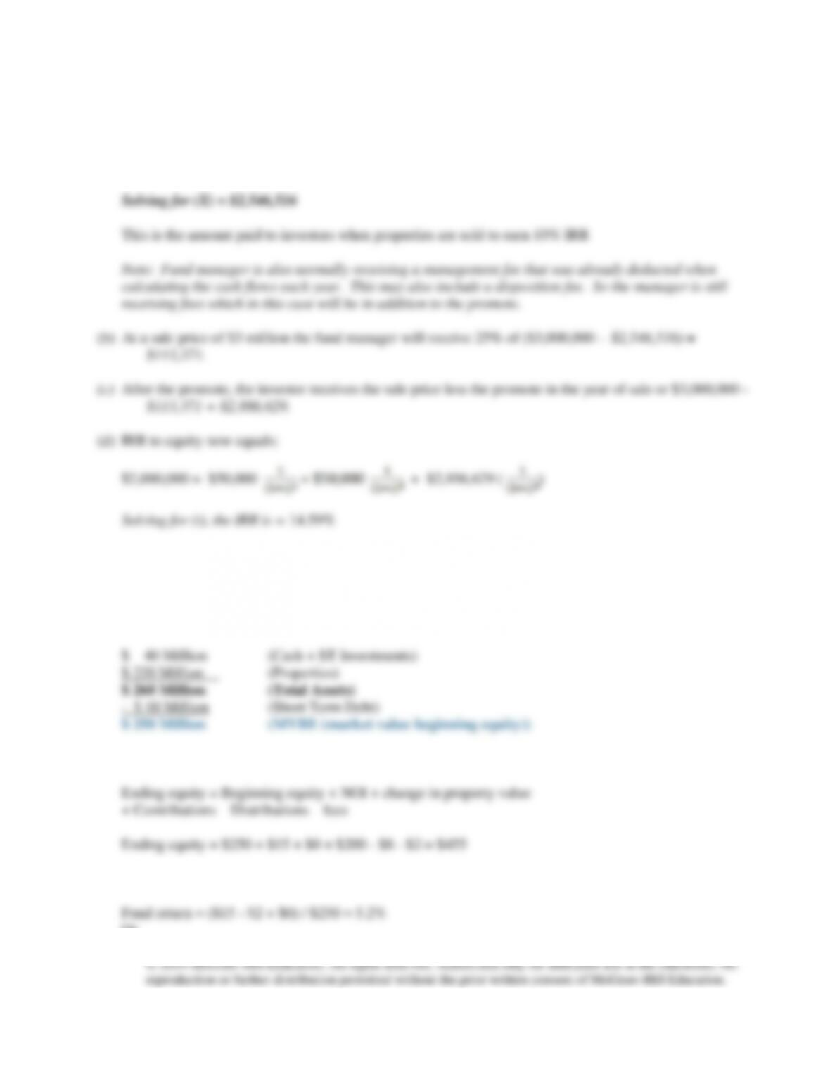
Target Return to Investors = 10% IRR, then a 25% promote is paid to manager
(a) $2,000,000 = $50,000 / (1.1) + $50,000 / (1.1)2 + X / (1.1)3
PROBLEM 23-3
Quarterly Fund Performance
(a) Beginning Equity:
(b) What is MVEE?
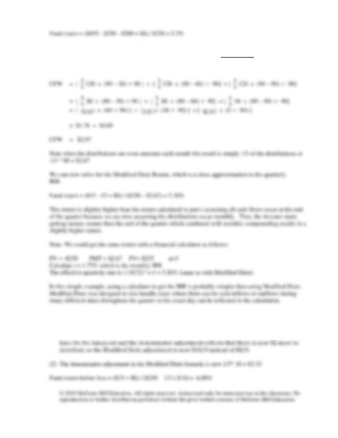
(c) If all cash flows occurred at the end of the quarter, the quarterly IRR for the fund would be:
Or
© 2019 McGraw-Hill Education. All rights reserved. Authorized only for instructor use in the classroom. No
reproduction or further distribution permitted without the prior written consent of McGraw-Hill Education.
Fund return = ($455 – $250 – $200 + $8) / $250 = 5.2%
(d) In cases when cash inflows and outflows occur many times during the quarter, rather than
performing an IRR calculation, the Modified Dietz Return (RD) is used to approximate the IRR:
First, solve for CFW to adjust the denominator in RD for timing of cash flows during the quarter:
(e) Returns “Before Fees”:
(1) Add back to distributions, the $2 million in fees paid to fund manager. This makes a total of
$10 million available for distributions “before fees”. So, the numerator to the return does not
(f) Returns at the “property level” would be determined by focusing only on those operating cash flows
related to properties in the fund and ignoring cash balances, leverage, fund fees, etc.
Note: NOI = $15 and is assumed to occur at the rate of $5 per month during the quarter. Also note that
(g) If we assume that properties in the fund would have appreciated to a total of $400 million by the end of
the quarter, we now have $30 appreciation in property values after adjusting for acquisitions. ($400 –
$220 – $150) = $30
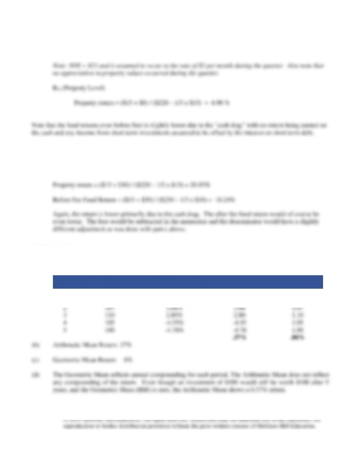
PROBLEM 23-4
Comparing IRR with Arithmetic Mean
(a)
Year
Fund Value
Annual Return
Arithmetic Mean Return
Cumulative Index
Value
0
100
0
0.00
1.00
1
103
3.00%
3.00
1.03
2
107
3.88%
3.88
1.07
3
110
2.80%
2.80
1.10
4
105
-4.55%
-4.55
1.05
5
100
-4.76%
-4.76
1.00
.37%
.00%
(b) Arithmetic Mean Return .37%
(c) Geometric Mean Return 0%
(d) The Geometric Mean reflects annual compounding for each period. The Arithmetic Mean does not reflect
any compounding of the return. Even though an investment of $100 would still be worth $100 after 5
years, and the Geometric Mean (IRR) is zero, the Arithmetic Mean shows a 0.37% return.
PROBLEM 23–5
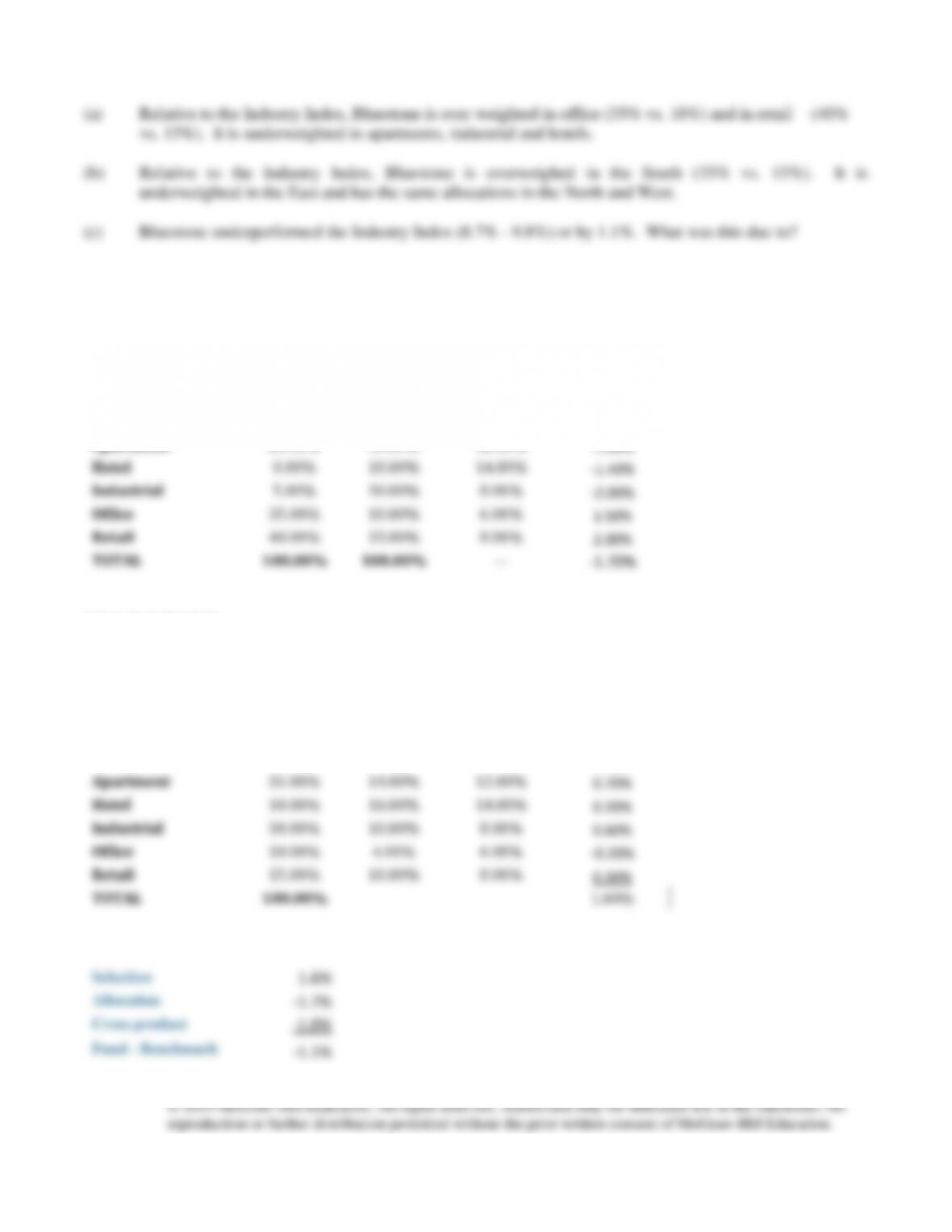
ATTRIBUTION ANALYSIS: Property Type
A L L O C A T I O N
Sector
Fund
Industry
Index
Industry
Index
Returns
Diff in weights
x Ind. Index
Ret.
Weights
Apartment
20.00%
35.00%
12.00%
-1.80%
Hotel
0.00%
10.00%
14.00%
-1.40%
Industrial
5.00%
30.00%
8.00%
-2.00%
Office
35.00%
10.00%
6.00%
1.50%
Retail
40.00%
15.00%
8.00%
2.00%
TOTAL
100.00%
100.00%
—
-1.70%
S E L E C T I O N
Sector
Industry
Index
Fund
Industry
Index
Weight
Returns
Diff in returns
x Benchmark
weight
Apartment
35.00%
14.00%
12.00%
0.70%
Hotel
10.00%
16.00%
14.00%
0.20%
Industrial
30.00%
10.00%
8.00%
0.60%
Office
10.00%
4.00%
6.00%
-0.20%
Retail
15.00%
10.00%
8.00%
0.30%
TOTAL
100.00%
1.60%
Selection
1.6%
Allocation
-1.7%
Cross product
-1.0%
Fund – Benchmark
-1.1%

ANALYSIS: The fund did a better job selecting individual properties but its allocation decision hurt its
performance. The interaction of the two was -1%.
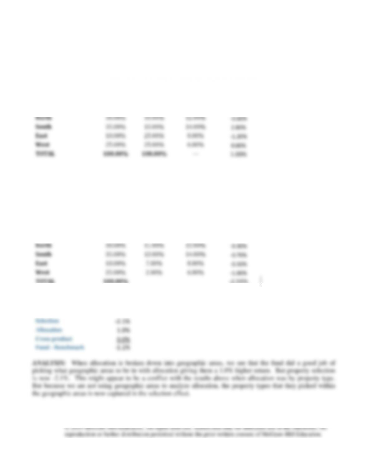
(d)
ATTRIBUTION ANALYSIS: Geographic Region
A L L O C A T I O N
Sector
Fund
Industry
Index
Industry
Index
Returns
Diff in weights
x Ind. Index
Ret.
Weights
North
30.00%
35.00%
12.00%
-0.60%
South
35.00%
15.00%
14.00%
2.80%
East
10.00%
25.00%
8.00%
-1.20%
West
25.00%
25.00%
6.00%
0.00%
TOTAL
100.00%
100.00%
—
1.00%
S E L E C T I O N
Sector
Industry
Index
Fund
Industry
Index
Weight
Returns
Diff in returns
x Benchmark
weight
North
30.00%
11.00%
12.00%
-0.30%
South
35.00%
12.00%
14.00%
-0.70%
East
10.00%
7.00%
8.00%
-0.10%
West
25.00%
2.00%
6.00%
-1.00%
TOTAL
100.00%
-2.10%
Summary
Selection
–2.1%
Allocation
1.0%
Cross product
0.0%
Fund – Benchmark
-1.1%
ANALYSIS: When allocation is broken down into geographic areas, we see that the fund did a good job of
picking what geographic areas to be in with allocation giving them a 1.0% higher return. But property selection
is now -2.1%. This might appear to be a conflict with the results above when allocation was by property type.
But because we are not using geographic areas to analyze allocation, the property types that they picked within
the geographic areas is now captured in the selection effect.
Another way we could have done this is to do the breakdown by combinations of region and division in a single
analysis, e.g. south apartments, south retail, etc. which would result in 5 property types times 4 regions or 20
different combinations with weights and returns for each to compare to the benchmark.
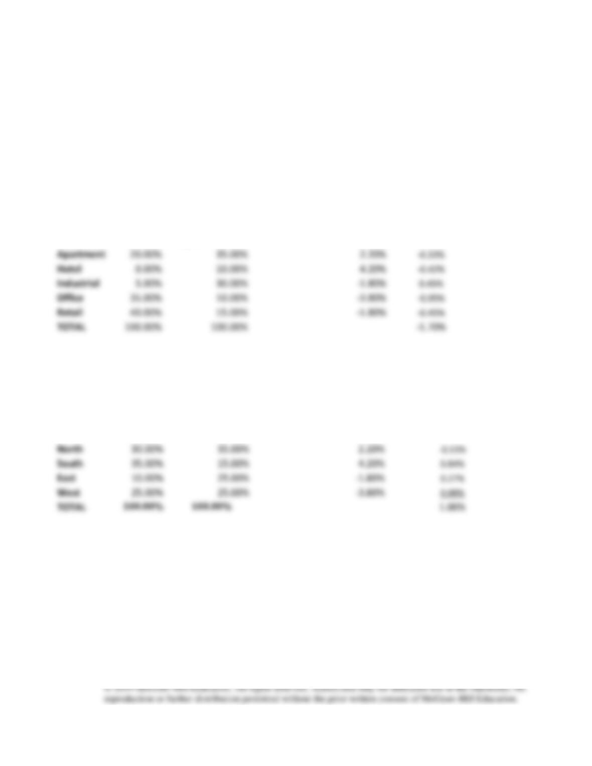
(e) The total allocation effect is the same at -1.70% but the contribution of each sector is now more meaningful
and indicates that all but the allocation to industrial hurt performance.
Brinson-Fachler
(BF)
Allocation Alternative Methodology
Sector
Fund
Benchmark
Benchmark Relative Return
=Sector Benchmark Returns
– Total Benchmark Return
Diff in weights
x Benchmark
Relative Return
Weights
Apartment
20.00%
35.00%
2.20%
-0.33%
Hotel
0.00%
10.00%
4.20%
-0.42%
Industrial
5.00%
30.00%
-1.80%
0.45%
Office
35.00%
10.00%
-3.80%
-0.95%
Retail
40.00%
15.00%
-1.80%
-0.45%
TOTAL
100.00%
100.00%
-1.70%
(f) The total allocation effect is the same at -1.70% but the contribution of each sector is now more meaningful
and indicates that all but the allocation to the North hurt performance.
Sector
Fund
Benchmark
Benchmark Relative Return
=Sector Benchmark Returns
– Total Benchmark Return
Diff in weights x
Benchmark Relative
Return
Weights
North
30.00%
35.00%
2.20%
-0.11%
South
35.00%
15.00%
4.20%
0.84%
East
10.00%
25.00%
-1.80%
0.27%
West
25.00%
25.00%
-3.80%
0.00%
TOTAL
100.00%
100.00%
1.00%