Unlock document.
This document is partially blurred.
Unlock all pages and 1 million more documents.
Get Access
Chapter 04 - Market Failures: Public Goods and Externalities
4-12
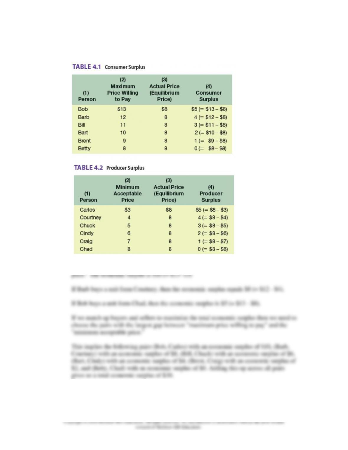
Feedback: Consider the following tables as an example:
If Bob buys a unit of the good from Carlos, then the economic surplus is the difference
between Bob's "maximum price willing to pay" and Carlos's the "minimum acceptable
Chapter 04 - Market Failures: Public Goods and Externalities
4-13
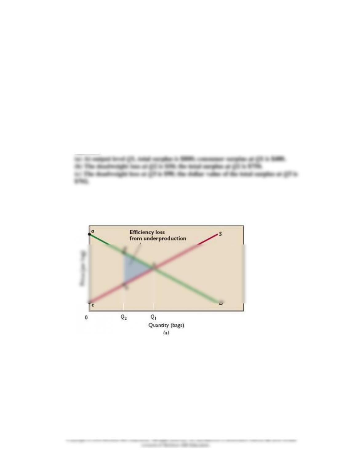
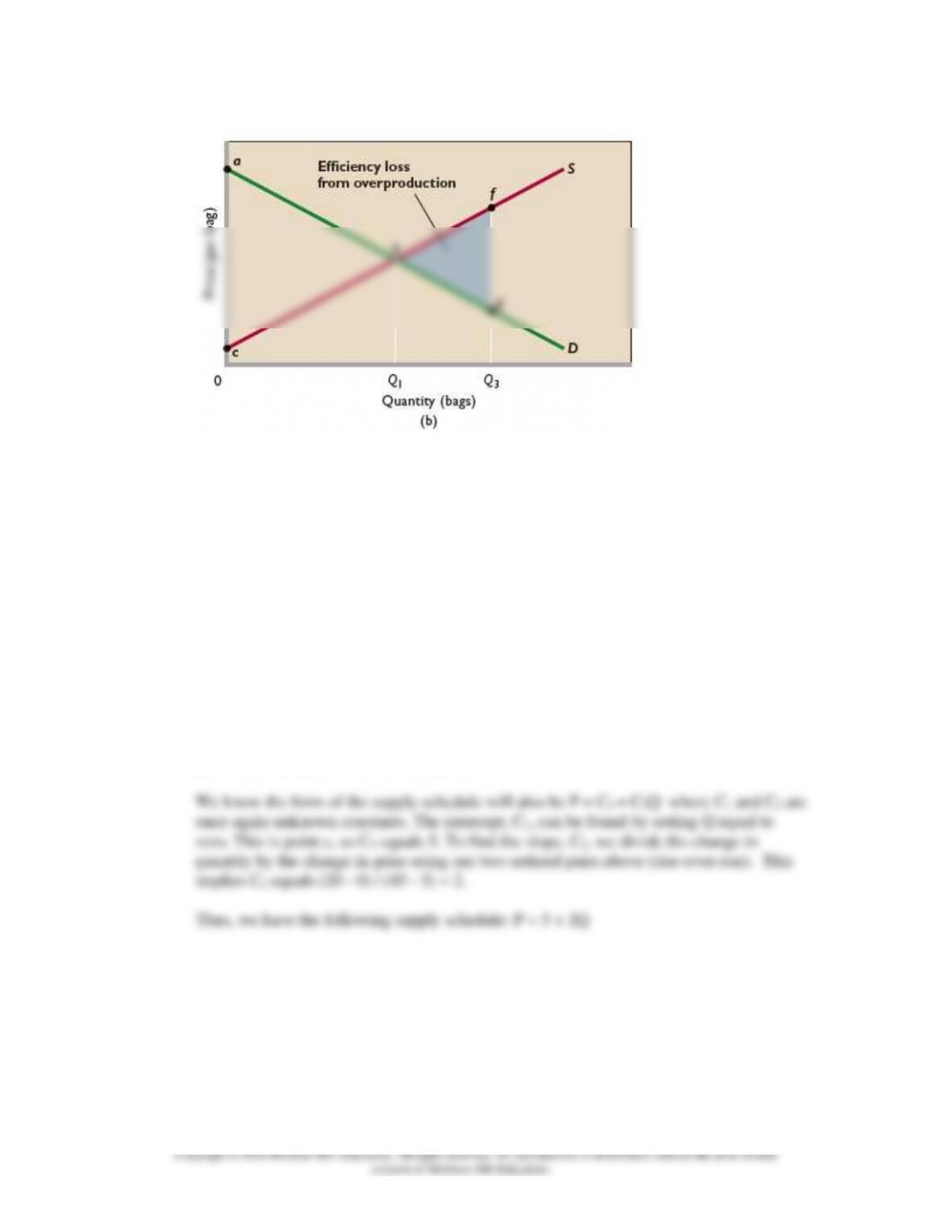
4. ADVANCED ANALYSIS Assume the following values for Figures 4.4a and 4.4b. Q1 = 20
bags. Q2 = 15 bags. Q3 = 27 bags. The market equilibrium price is $45 per bag. The price at a is
$85 per bag. The price at c is $5 per bag. The price at f is $59 per bag. The price at g is $31 per
bag. Apply the formula for the area of a triangle (Area = ½ x Base x Height) to answer the
following questions. LO2
a. What is the dollar value of the total surplus (producer surplus plus consumer surplus) when the
allocatively efficient output level is being produced? How large is the dollar value of the
consumer surplus at that output level?
b. What is the dollar value of the deadweight loss when output level Q2 is being produced? What
is the total surplus when output level Q2 is being produced?
c. What is the dollar value of the deadweight loss when output level Q3 is produced? What is the
dollar value of the total surplus when output level Q3 is produced?
Answers:
Feedback: To answer this question, let us first find the mathematical representation of
the supply and demand schedules. To help us accomplish this objective we us the
following figures.
Chapter 04 - Market Failures: Public Goods and Externalities
4-14
Now consider the following values as an example. Assume the following values for
Figures 5.4a and 5.4b: The equilibrium quantity Q1 = 20, the market equilibrium price is
$45 per bag, the price at a is $85 per bag, the price at c is $5 per bag.
To derive the demand schedule (inverse demand schedule), we use the following ordered
pairs: (20,45) equilibrium and (0,85) point a.
We know the form of the demand schedule will be P=C1 + C2Q where C1 and C2 are
unknown constants. The intercept, C1, can be found by setting Q equal to zero. This is
point a, so C1 equals 85. To find the slope, C2, we divide the change in quantity by the
change in price using our two ordered pairs above (rise-over-run). This implies C2 equals
(20 - 0) / (45 - 85) = -2.
Thus, we have the following demand schedule: P = 85 - 2Q
To derive the supply schedule (inverse supply schedule), we use the following ordered
pairs: (20,45) equilibrium and (0,5) point c.
Chapter 04 - Market Failures: Public Goods and Externalities
4-15
With these schedules we can now answer the following questions:
Part (a): What is the dollar value of the total surplus (producer surplus plus consumer
surplus) when the allocatively efficient output level is being produced? How large is the
dollar value of the consumer surplus at that output level?
To calculate total surplus we use the following formula for the area of a triangle (Area =
½ (Base x Height)).
The area between the demand schedule P = 85 - 2Q and the supply schedule P = 5 + 2Q
Part (b): What is the dollar value of the deadweight loss when output level Q2 is being
produced? What is the total surplus when output level Q2 is being produced?
The total surplus can be found by subtracting the deadweight loss from the original total
surplus that maximized efficiency. This is 800 (maximum total surplus) - 50 (deadweight
loss) = 750.
Part (c): What is the dollar value of the deadweight loss when output level Q3 is
produced? What is the dollar value of the total surplus when output level Q3 is produced?
Here we follow the same procedure. We are given the price at point f is $59 and the price
at point g is $31 (we do not need to calculate these prices using the demand and supply
Chapter 04 - Market Failures: Public Goods and Externalities
4-16
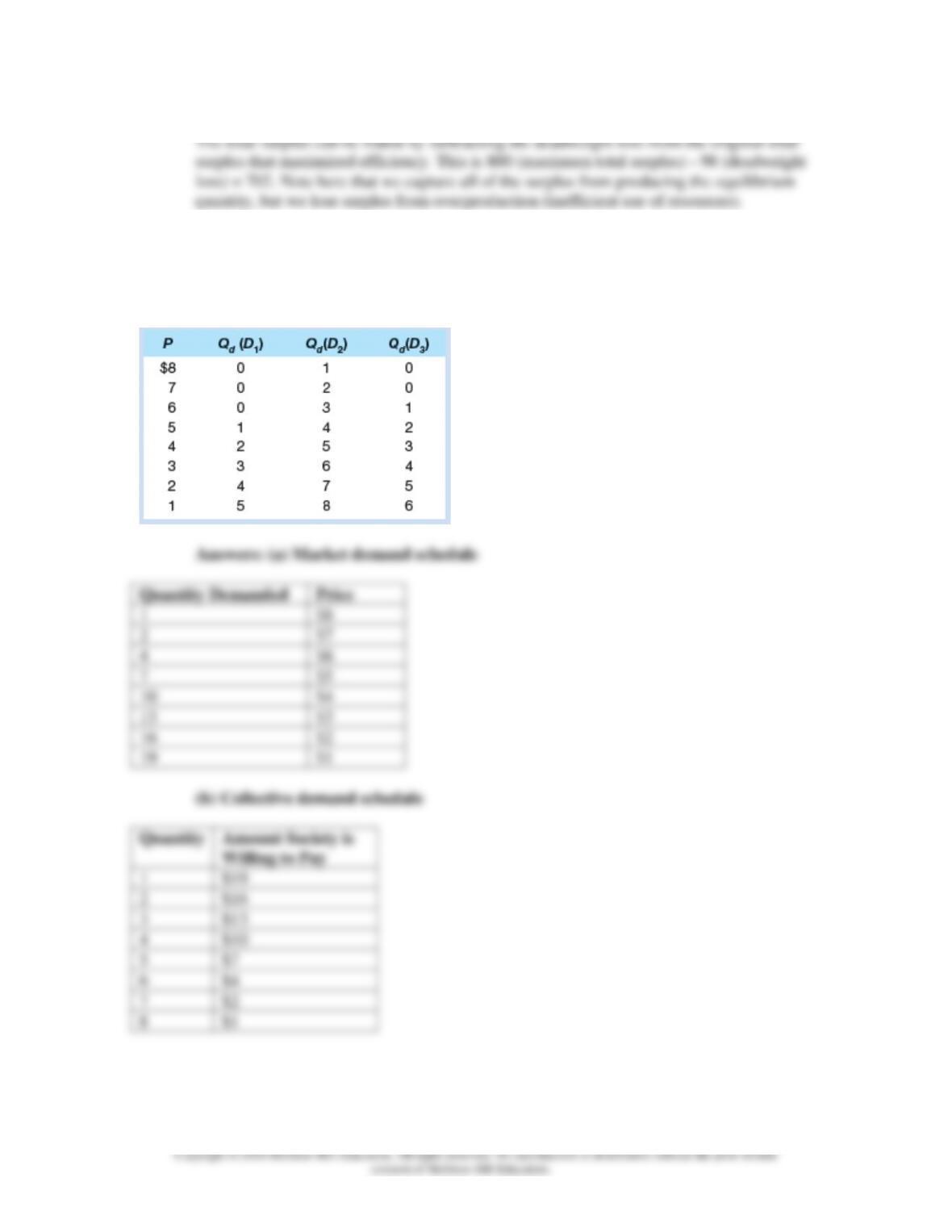
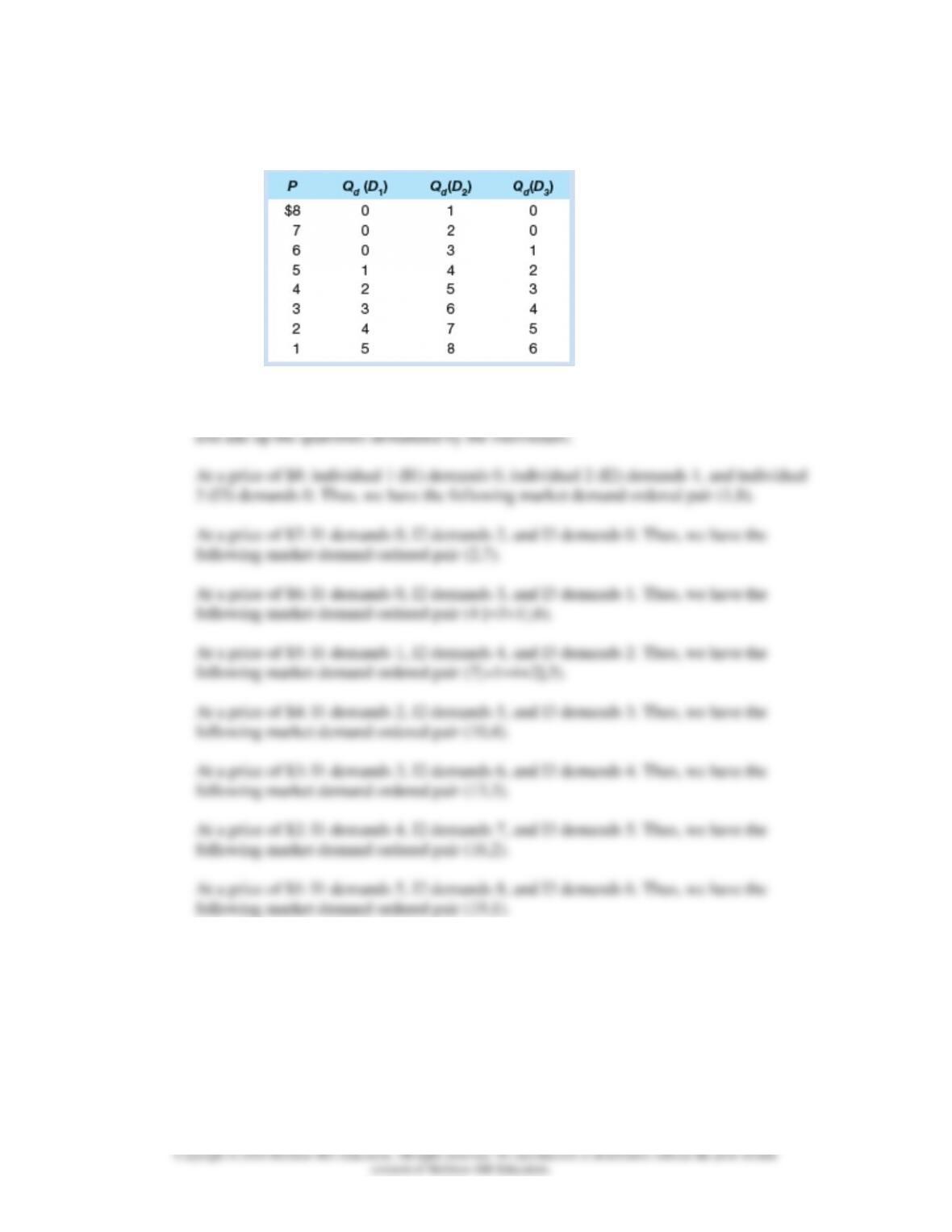
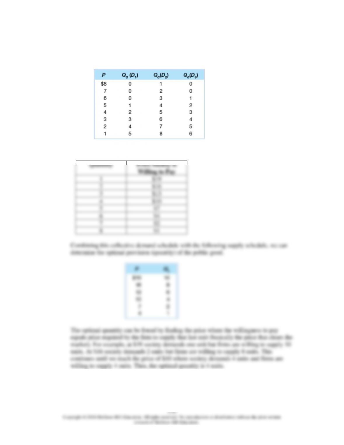
5. On the basis of the three individual demand schedules below, and assuming these three people
are the only ones in the society, determine (a) the market demand schedule on the assumption that
the good is a private good and (b) the collective demand schedule on the assumption that the good
is a public good. LO3
Chapter 04 - Market Failures: Public Goods and Externalities
4-17
Feedback: Consider the following table:
Part (a): Derive the market demand schedule on the assumption that the good is a private
good. To accomplish we use the principle of horizontal summation. That is, we fix price
Chapter 04 - Market Failures: Public Goods and Externalities
4-18
Part (b): Derive the collective demand schedule on the assumption that the good is a
public good. To accomplish we use the principle of vertical summation. That is, we fix
quantity and add up the price (willingness to pay) for the individuals. The logic here is
that the individuals (society) can pool resources to purchase a given quantity because this
good will be shared (public good).
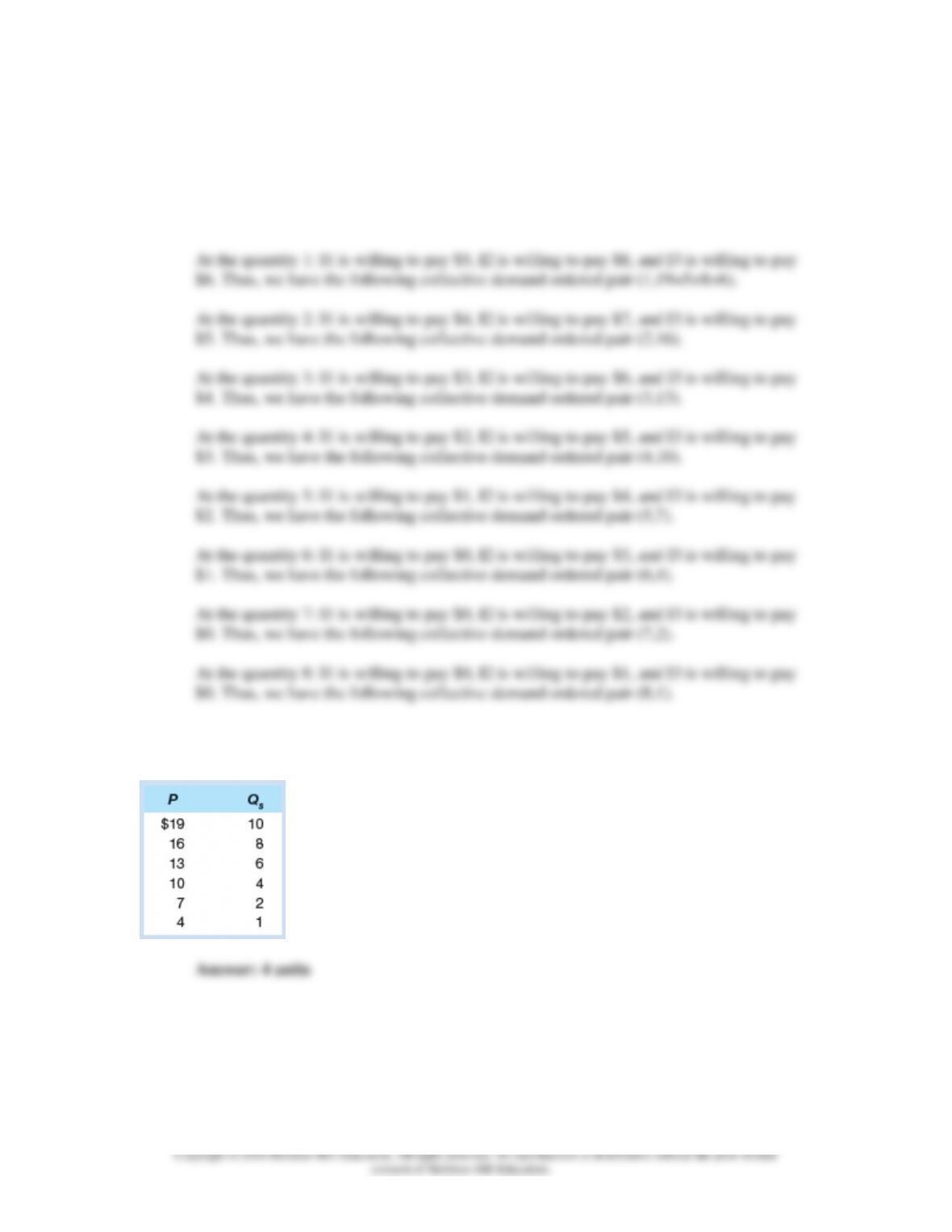
6. Use your demand schedule for a public good, determined in problem 5, and the following
supply schedule to ascertain the optimal quantity of this public good. LO3
Chapter 04 - Market Failures: Public Goods and Externalities
Feedback: From the example table in problem 5, we calculated the collective demand
schedule from the individual demand schedules:
Collective Demand Schedule:
Quantity
Price Society is
Willing to Pay
1
$19
2
$16
3
$13
4
$10
5
$7
6
$4
7
$2
8
$1
Combining this collective demand schedule with the following supply schedule, we can
determine the optimal provision (quantity) of the public good.
The optimal quantity can be found by finding the price where the willingness to pay
equals price required by the firm to supply that last unit (basically the price that clears the
market). For example, at $19 society demands one unit but firms are willing to supply 10
units. At $16 society demands 2 units but firms are willing to supply 8 units. This
continues until we reach the price of $10 where society demands 4 units and firms are
willing to supply 4 units. Thus, the optimal quantity is 4 units.
4-20
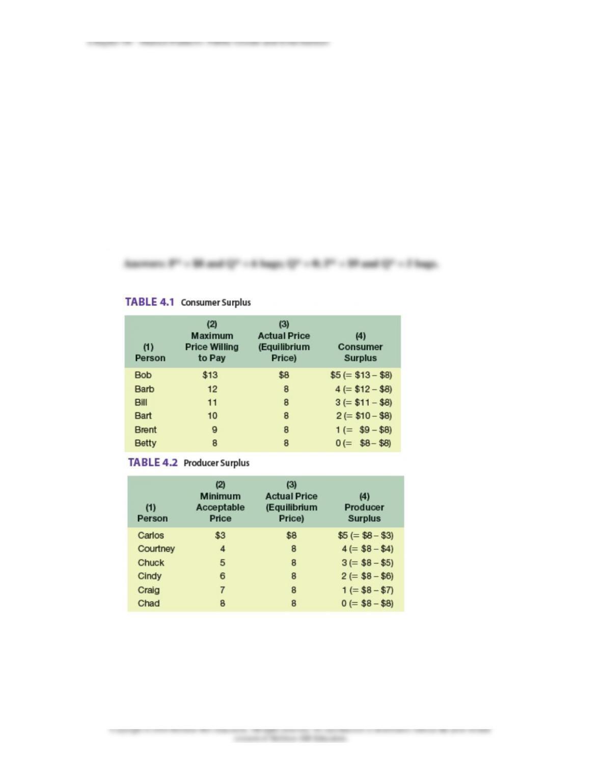
7. Look at Tables 4.1 and 4.2, which show, respectively, the willingness to pay and willingness to
accept of buyers and seller of bags of oranges. For the following questions, assume that the
equilibrium price and quantity will depend on the indicated changes in supply and demand.
Assume that the only market participants are those listed by name in the two tables. LO4
a. What are the equilibrium price and quantity for the data displayed in the two tables?
b. What if instead of bags of oranges, the data in the two tables dealt with a public good like
fireworks displays. If all the buyers free ride, what will be the quantity supplied by private
sellers?
c. Assume that we are back to talking about bags of oranges (a private good), but that the
government has decided that tossed orange peels impose a negative externality on the public that
must be rectified by imposing a $2-per-bag tax on sellers. What is the new equilibrium price and
quantity? If the new equilibrium quantity is the optimal quantity, by how many bags were oranges
being overproduced before?
Feedback: Here we consider the tables from Problems 1 and 2.
Chapter 04 - Market Failures: Public Goods and Externalities
4-21
Part (a): To determine the equilibrium price of oranges, we begin by comparing the
highest willingness to pay with the lowest minimum acceptable price. Bob is willing to
pay $13 and Carlos is willing to accept at minimum $3. This trade is made because Bob
Part (c): If the government decides that tossed orange peels impose a negative externality
on the public that must be rectified by imposing a $2-per-bag tax on sellers, then the
"minimum acceptable price" will increase by the amount of the tax. The reason is that the
Bob is willing to pay $13 and Carlos is willing to accept at minimum $5. This trade is
made because Bob is willing to pay more than Carlos requires for the sale. We then move
on to the trade between Barb and Courtney. This trade is also made because Barb is


