978-1259723223 Chapter 38

subject Type Homework Help
subject Pages 9
subject Words 4454
subject Authors Campbell McConnell, Sean Flynn, Stanley Brue

Unlock document.

This document is partially blurred.
Unlock all pages and 1 million more documents.
Get Access
page-pf1
Chapter 38 - Extending the Analysis of Aggregate Supply
38-1
Chapter 38 - Extending the Analysis of Aggregate Supply
McConnell Brue Flynn 21e
DISCUSSION QUESTIONS
1. Distinguish between the short run and the long run as they relate to macroeconomics. Why is
the distinction important? LO1
2. Which of the following statements are true? Which are false? Explain why the false statements
are untrue. LO1
a. Short-run aggregate supply curves reflect an inverse relationship between the price level and
the level of real output.
b. The long-run aggregate supply curve assumes that nominal wages are fixed.
c. In the long run, an increase in the price level will result in an increase in nominal wages.
3. Suppose the government misjudges the natural rate of unemployment to be much lower than it
actually is, and thus undertakes expansionary fiscal and monetary policies to try to achieve the
lower rate. Use the concept of the short-run Phillips Curve to explain why these policies might at
first succeed. Use the concept of the long-run Phillips Curve to explain the long-run outcome of
these policies. LO4
page-pf2
Chapter 38 - Extending the Analysis of Aggregate Supply
38-2
Copyright © 2018 McGraw-Hill Education. All rights reserved. No reproduction or distribution without the prior written
consent of McGraw-Hill Education.
Answer: In the short-run there is probably a tradeoff between unemployment and
inflation. The government’s expansionary policy should reduce unemployment as
aggregate demand increases. However, the government has misjudged the natural rate
and will continue its expansionary policy beyond the point of the natural level of
unemployment. As aggregate demand continues to rise, prices begin to rise. In the long-
run, workers demand higher wages to compensate for these higher prices. Aggregate
supply will decrease (shift leftward) toward the natural rate of unemployment.
In other words, any reduction of unemployment below the natural rate is only temporary
and involves a short-run rise in inflation. This, in turn, causes long-run costs to rise and a
decrease in aggregate supply. The end result should be an equilibrium at the natural rate
of unemployment and a higher price level than the beginning level. The long-run Phillips
curve is thus a vertical line connecting the price levels possible at the natural rate of
unemployment found on the horizontal axis.
4. What do the distinctions between short-run aggregate supply and long-run aggregate supply
have in common with the distinction between the short-run Phillips Curve and the long-run
Phillips Curve? Explain. LO4
5. What is the Laffer Curve, and how does it relate to supply-side economics? Why is
determining the economy’s location on the curve so important in assessing tax policy? LO5
page-pf3
Chapter 38 - Extending the Analysis of Aggregate Supply
38-3
6.Why might one person work more, earn more, and pay more income tax when his or her tax
rate is cut, while another person will work less, earn less, and pay less income tax under the same
circumstance? LO5
7. LAST WORD On average, does an increase in taxes raise or lower real GDP? If taxes as a
percent of GDP go up 1 percent, by how much does real GDP change? Are the decreases in real
GDP caused by tax increases temporary or permanent? Does the intention of a tax increase
matter?
REVIEW QUESTIONS
1. Suppose the full-employment level of real output (Q) for a hypothetical economy is $250 and
the price level (P) initially is 100. Use the short-run aggregate supply schedules below to answer
the questions that follow: LO1
a. What will be the level of real output in the short run if the price level unexpectedly rises from
100 to 125 because of an increase in aggregate demand? What if the price level unexpectedly falls
from 100 to 75 because of a decrease in aggregate demand? Explain each situation, using
numbers from the table.
b. What will be the level of real output in the long run when the price level rises from 100 to 125?
When it falls from 100 to 75? Explain each situation.
c. Show the circumstances described in parts a and b on graph paper, and derive the long-run
aggregate supply curve.
page-pf4
Chapter 38 - Extending the Analysis of Aggregate Supply
38-4
Answer:
2. Suppose that AD and AS intersect at an output level that is higher than the full-employment
output level. After the economy adjusts back to equilibrium in the long run, the price level will be
__________ . LO2
a. Higher than it is now.
b. Lower than it is now.
c. The same as it is now.
page-pf5
Chapter 38 - Extending the Analysis of Aggregate Supply
38-5
3. Suppose that an economy begins in long-run equilibrium before the price level and real GDP
both decline simultaneously. If those changes were caused by only one curve shifting, then those
changes are best explained as the result of: LO2
a. The AD curve shifting right.
b. The AS curve shifting right.
c. The AD curve shifting left.
d. The AS curve shifting left.
4. Identify the two descriptions below as being the result of either cost-push inflation or demand-
pull inflation. LO2
a. Real GDP is below the full-employment level and prices have risen recently.
b. Real GDP is above the full-employment level and prices have risen recently.
page-pf6
Chapter 38 - Extending the Analysis of Aggregate Supply
38-6
5. Use graphical analysis to show how each of the following would affect the economy first in the
short run and then in the long run. Assume that the United States is initially operating at its full-
employment level of output, that prices and wages are eventually flexible both upward and
downward, and that there is no counteracting fiscal or monetary policy. LO2
a. Because of a war abroad, the oil supply to the United States is disrupted, sending oil prices
rocketing upward.
b. Construction spending on new homes rises dramatically, greatly increasing total U.S.
investment spending.
c. Economic recession occurs abroad, significantly reducing foreign purchases of U.S. exports.
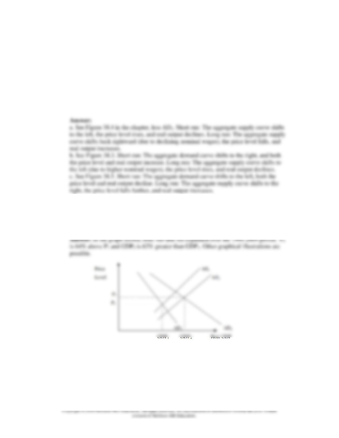
6. Between 1990 and 2009, the U.S. price level rose by about 64 percent while real output
increased by about 62 percent. Use the aggregate demandaggregate supply model to illustrate
these outcomes graphically. LO2
Answer: In the graph shown, both AD and AS expanded over the 1990-2009 period. P2
page-pf7
Chapter 38 - Extending the Analysis of Aggregate Supply
38-7
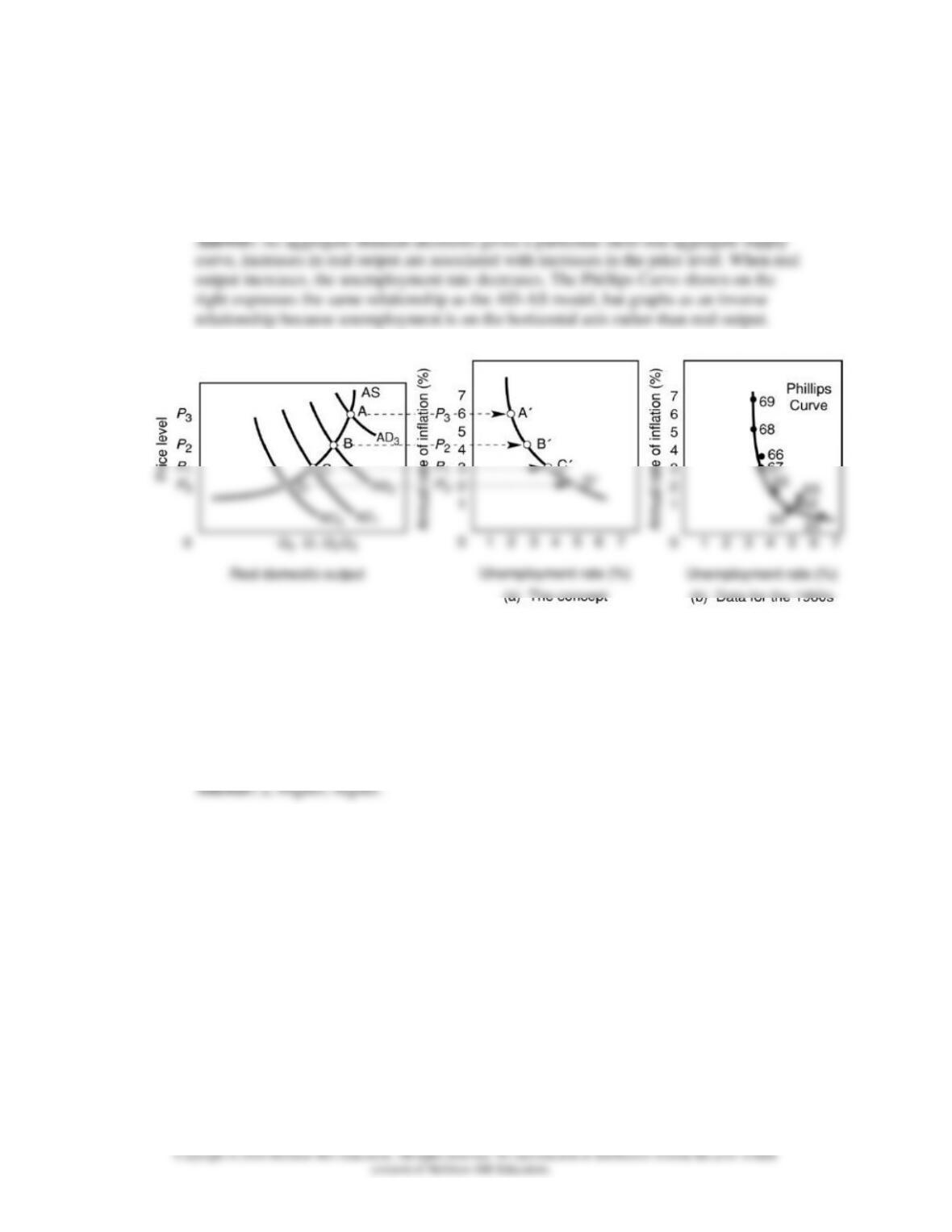
7. Assume there is a particular short-run aggregate supply curve for an economy and the curve is
relevant for -several years. Use the AD-AS analysis to show graphically why higher rates of
inflation over this period would be associated with lower rates of unemployment, and vice versa.
What is this inverse relationship called? LO3
8. Aggregate supply shocks can cause ________ rates of inflation that are accompanied by
________ rates of unemployment. LO3
a. Higher; higher.
b. Higher; lower.
c. Lower; higher.
d. Lower; lower.
page-pf8
Chapter 38 - Extending the Analysis of Aggregate Supply
38-8
Feedback: The correct answer is that aggregate supply shocks can cause higher rates of
inflation that are accompanied by higher rates of unemployment.
9. Suppose that firms are expecting 6 percent inflation while workers are expecting 9 percent
inflation. How much of a pay raise will workers demand if their goal is to maintain the
purchasing power of their incomes? LO4
a. 3 percent.
b. 6 percent.
c. 9 percent.
d. 12 percent.
page-pf9
Chapter 38 - Extending the Analysis of Aggregate Supply
38-9
10. Suppose that firms were expecting inflation to be 3 percent, but then it actually turned out to
be 7 percent. Other things equal, firm profits will be: LO4
a. Smaller than expected.
b. Larger than expected.
PROBLEMS
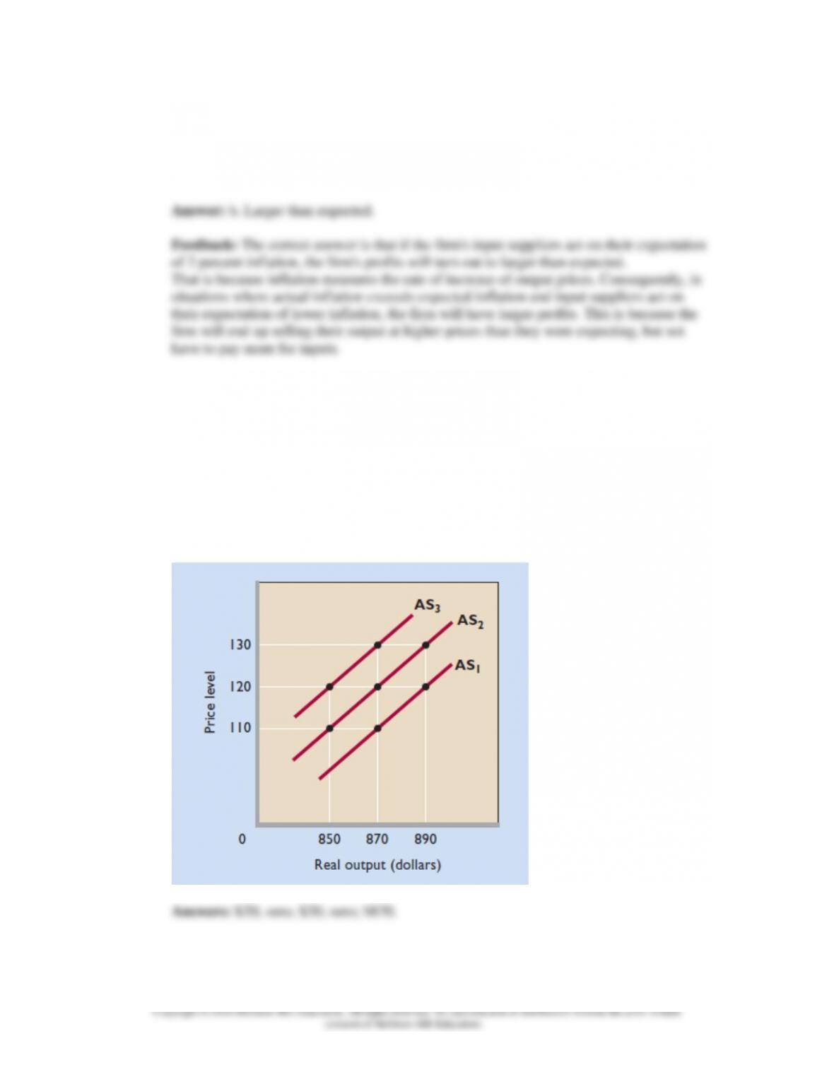
1. Use the accompanying figure to answer the follow questions. Assume that the economy
initially is operating at price level 120 and real output level $870. This output level is the
economy’s potential (or full-employment) level of output. Next, suppose that the price level rises
from 120 to 130. By how much will real output increase in the short run? In the long-run?
Instead, now assume that the price level dropped from 120 to 110. Assuming flexible product and
resource prices, by how much will real output fall in the short run? In the long run? What is the
long-run level of output at each of the three price levels shown? LO1
page-pfa
Chapter 38 - Extending the Analysis of Aggregate Supply
38-10
Feedback:
The economy is initially operating at the price level 120 and real output level $870 (on
AS2). This output level is also the economy’s potential (or full-employment) level of
output.
Next, suppose that the price level rises from 120 to 130. By how much will real output
Instead, now assume that the price level dropped from 120 to 110. Assuming flexible
product and resource prices, by how much will real output fall in the short run? In the
What is the long-run level of output at each of the three price levels shown?
2. ADVANCED ANALYSIS Suppose that the equation for a particular short-run AS curve is P
= 20 + .5Q, where P is the price level and Q is real output in dollar terms. What is Q if the price
level is 120? Suppose that the Q in your answer is the full-employment level of output. By how
much will Q increase in the short run if the price level unexpectedly rises from 120 to 132? By
how much will Q increase in the long-run due to the price level increase? LO1
page-pfb
Chapter 38 - Extending the Analysis of Aggregate Supply
38-11
3. Suppose that over a 30-year period Buskerville’s price level increased from 72 to 138 while its
real GDP rose from $1.2 trillion to $2.1 trillion. Did economic growth occur in Buskerville? If so,
by what average yearly rate? Did Buskerville experience inflation? If so, by what average yearly
rate? Which shifted rightward faster in Buskerville: its long-run aggregate supply curve (ASLR)
or its aggregate demand curve (AD)? LO2
4. Suppose that for years East Confetti’s short-run Phillips Curve was such that each 1 percentage
point increase in its unemployment rate was associated with a 2 percentage point decline in its
inflation rate. Then, during several recent years the short run pattern changed such that its
inflation rate rose by 3 percentage points for every 1 percentage point drop in its unemployment
rate. Graphically, did East Confetti’s Phillips Curve shift upward or did it shift downward? LO3

Trusted by Thousands of
Students

Here are what students say about us.

Copyright ©2022 All rights reserved. | CoursePaper is not sponsored or endorsed by any college or university.