Chapter 01 Appendix
Chapter 01 Appendix
McConnell Brue Flynn 21e
APPENDIX DISCUSSION QUESTIONS
1. Briefly explain the use of graphs as a way to represent economic relationships. What is an
inverse relationship? How does it graph? What is a direct relationship? How does it graph? LO8
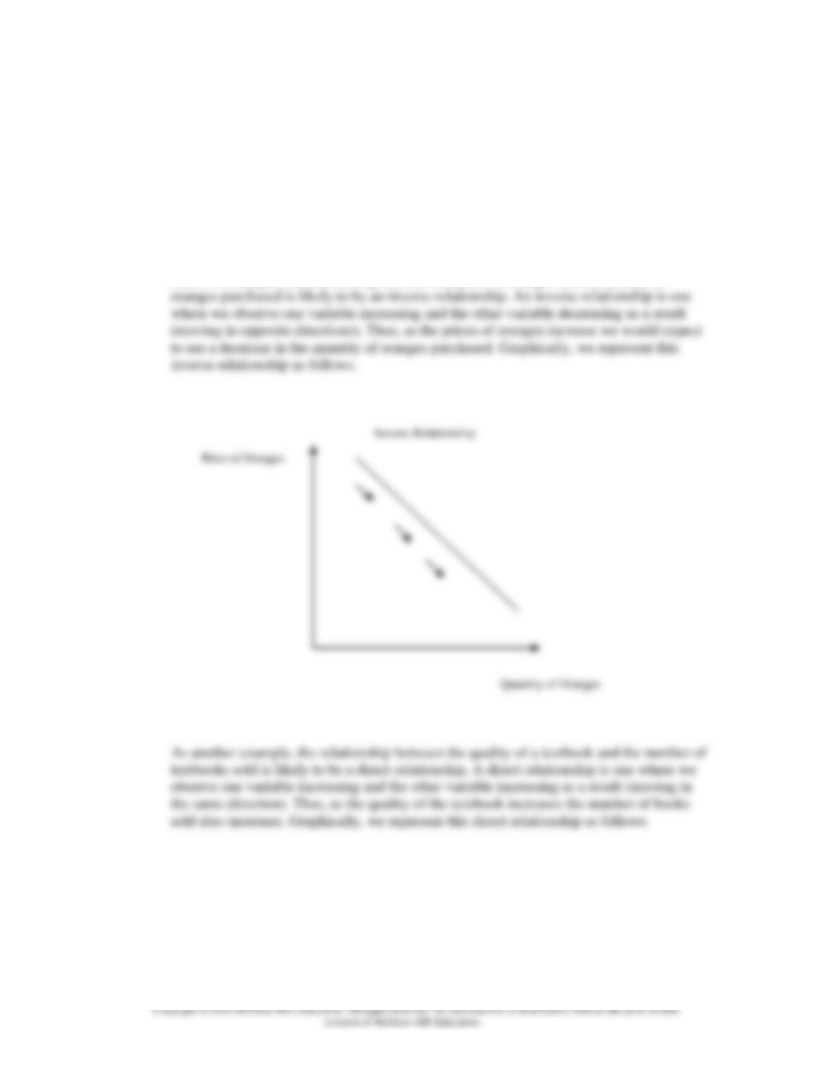
Answer: Graphs help us visualize relationships between key economic variables in the
data. For example, the relationship between the price of oranges and the number of
Chapter 01 Appendix
2. Describe the graphical relationship between ticket prices and the number of people choosing to
visit amusement parks. Is that relationship consistent with the fact that, historically, park
attendance and ticket prices have both risen? Explain. LO8
Answer: There is likely an inverse relationship between ticket prices and the number of
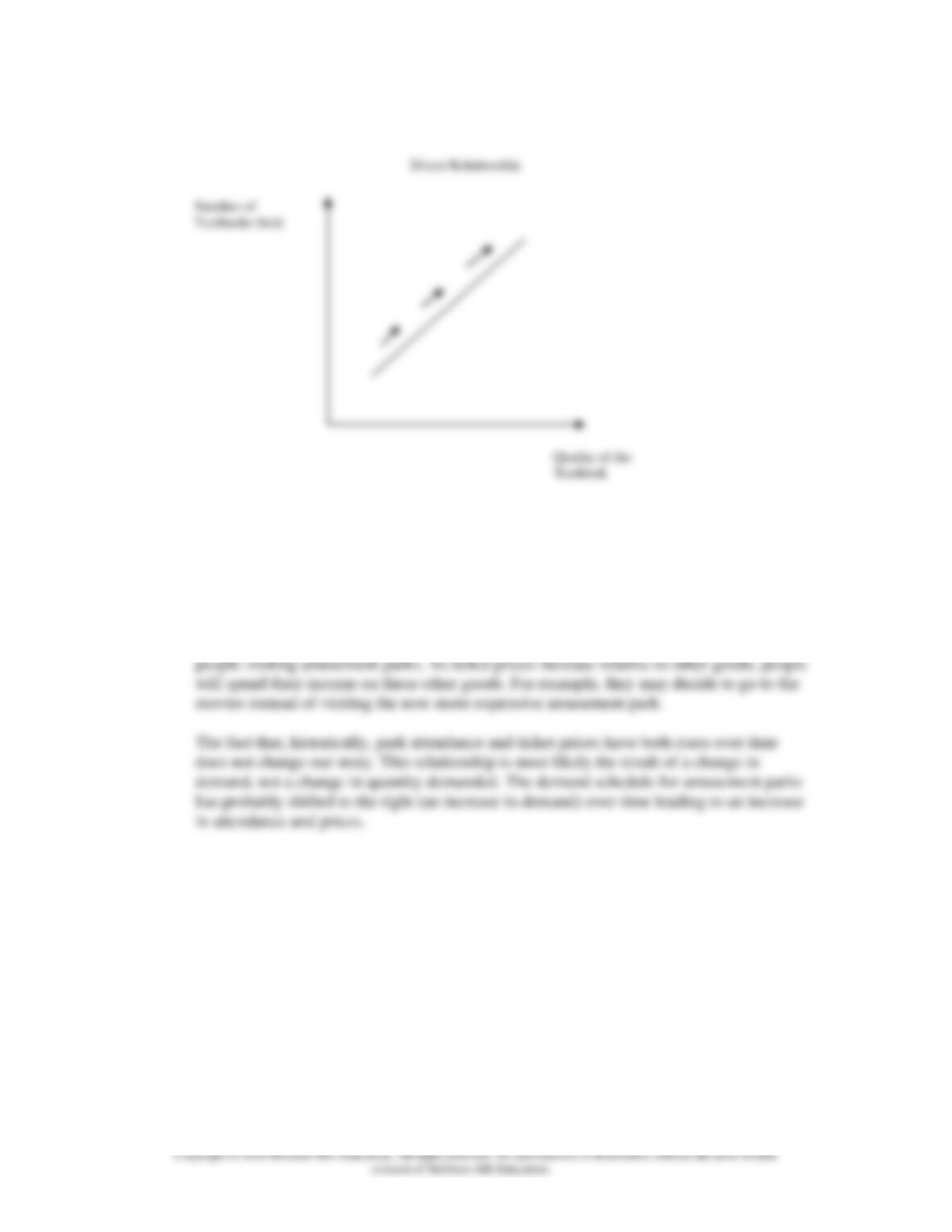
Number of
Textbooks Sold
Quality of the
Textbook
Direct Relationship
Chapter 01 Appendix
1A-3
3. Look back at Figure 2, which shows the inverse relationship between ticket prices and game
attendance at Gigantic State University. (a) Interpret the meaning of both the slope and the
intercept. (b) If the slope of the line were steeper, what would that say about the amount by which
ticket sales respond to increases in ticket prices? (c) If the slope of the line stayed the same but
the intercept increased, what can you say about the amount by which ticket sales respond to
increases in ticket prices? LO8
Answer:
Part a: The slope of this relationship tells us how much the price of a ticket must fall to
induce someone to buy an additional ticket. In this case, the slope of –2.5 tells us that the
price must fall by $2.50 to sell one more ticket (or to induce someone to buy one more
APPENDIX REVIEW QUESTIONS
1. Indicate whether each of the following relationships is usually a direct relationship or
an inverse relationship. LO8
a. A sports team’s winning percentage and attendance at its home games.
b. Higher temperature and sweater sales.
c. A person’s income and how often they shop at discount stores.
d. Higher gasoline prices and miles driven in automobiles.
Answer:
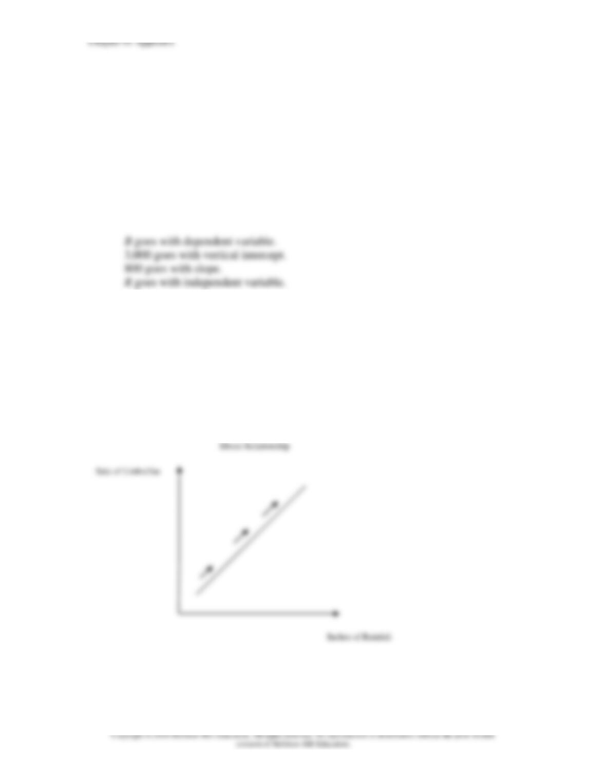
2. Erin grows pecans. The number of bushels (B) that she can produce depends on the
number of inches of rainfall (R) that her orchards get. The relationship is given
algebraically as follows: B = 3,000 + 800R. Match each part of this equation with the
correct term. LO8
B slope
3,000 dependent variable
800 vertical intercept
R independent variable
Answer:
APPENDIX PROBLEMS
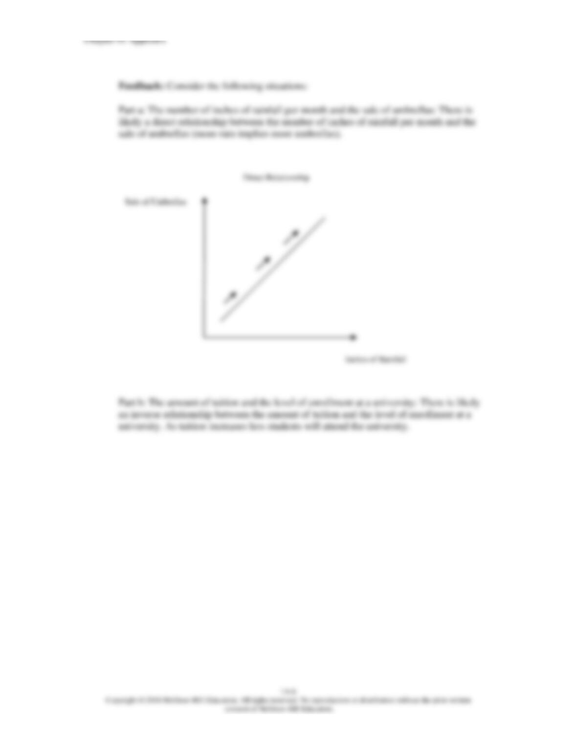
1. Graph and label as either direct or indirect the relationships you would expect to find between
(a) the number of inches of rainfall per month and the sale of umbrellas, (b) the amount of tuition
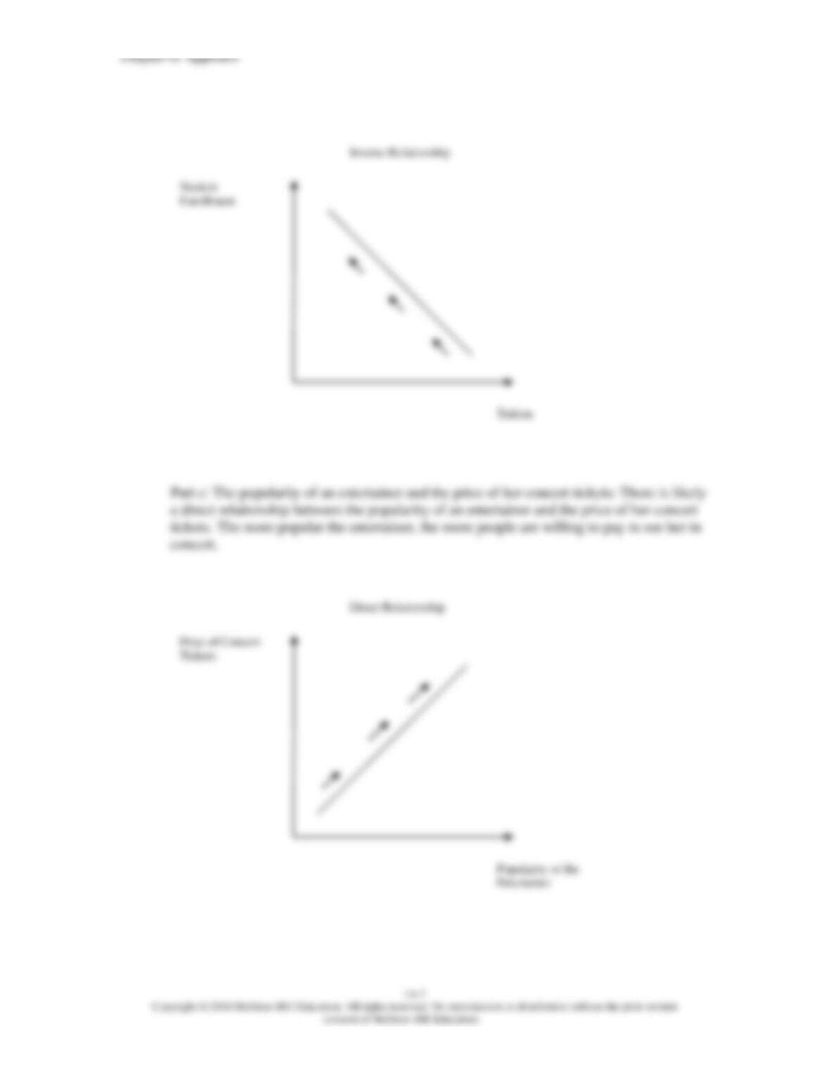
and the level of enrollment at a university, and (c) the popularity of an entertainer and the price of
her concert tickets. LO8
Answer:
Part a:
Sale of Umbrellas
Inches of Rainfall
Direct Relationship
Chapter 01 Appendix
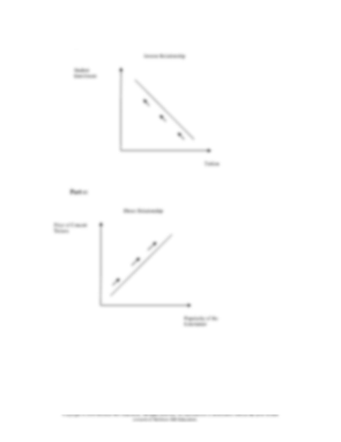
Part b:
Direct Relationship
Student
Enrollment
Tuition
Inverse Relationship
1A-8
2. Indicate how each of the following might affect the data shown in the table and graph in
Figure 2 of this appendix: LO8
a. GSU’s athletic director schedules higher-quality opponents.
b. An NBA team locates in the city where GSU plays.
c. GSU contracts to have all its home games televised.
Feedback: Consider the three scenarios:
1A-9
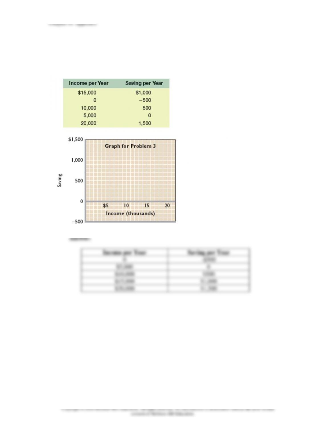
3. The following table contains data on the relationship between saving and income. Rearrange
these data into a logical order and graph them on the accompanying grid. What is the slope of the
line? The vertical intercept? Write the equation that represents this line. What would you predict
saving to be at the $12,500 level of income? LO8
Answer:
Chapter 01 Appendix
1A–10
Copyright © 2018 McGraw-Hill Education. All rights reserved. No reproduction or distribution without the prior written
consent of McGraw-Hill Education.
Slope equals (500/5000) or 0.10; the vertical intercept equals -$500. The equation
representing this data is : Saving = -$500 + 0.1 x Income. The predicted level of
saving is $750.
Feedback: Consider the following data:
Income per Year
Saving per Year
$15,000
$1,000
0
–$500
$10,000
$500
$5,000
0
$20,000
$1,500
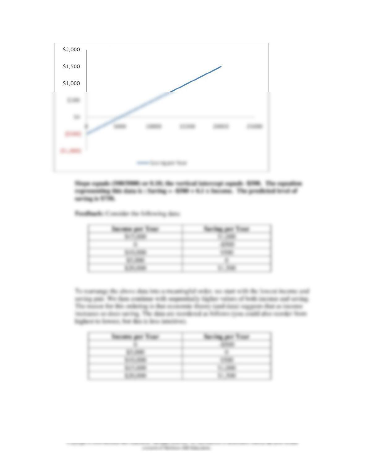
To rearrange the above data into a meaningful order, we start with the lowest income and
saving pair. We then continue with sequentially higher values of both income and saving.
The reason for this ordering is that economic theory (and data) suggests that as income
increases so does saving. The data are reordered as follows (you could also reorder from
highest to lowest, but this is less intuitive).
Income per Year
Saving per Year
0
–$500
$5,000
0
$10,000
$500
$15,000
$1,000
$20,000
$1,500
Chapter 01 Appendix
1A–11
Copyright © 2018 McGraw-Hill Education. All rights reserved. No reproduction or distribution without the prior written
consent of McGraw-Hill Education.
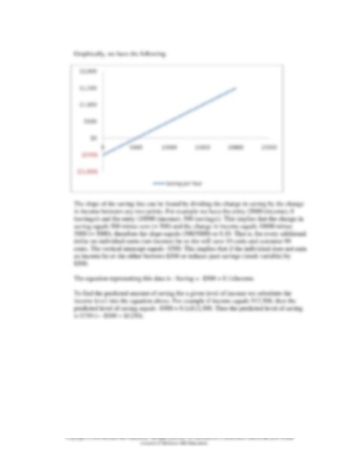
Graphically, we have the following.
The slope of the saving line can be found by dividing the change in saving by the change
in income between any two points. For example we have the entry (5000 (income), 0
(savings)) and the entry (10000 (income), 500 (savings)). This implies that the change in
saving equals 500 minus zero (= 500) and the change in income equals 10000 minus
5000 (= 5000), therefore the slope equals (500/5000) or 0.10. That is, for every additional
dollar an individual earns (net income) he or she will save 10 cents and consume 90
cents. The vertical intercept equals -$500. This implies that if the individual does not earn
an income he or she either borrows $500 or reduces past savings (stock variable) by
$500.
The equation representing this data is : Saving = -$500 + 0.1xIncome.
To find the predicted amount of saving for a given level of income we substitute the
income level into the equation above. For example if income equals $12,500, then the
predicted level of saving equals -$500 + 0.1x$12,500. Thus the predicted level of saving
is $750 (= -$500 + $1250).

1A–12
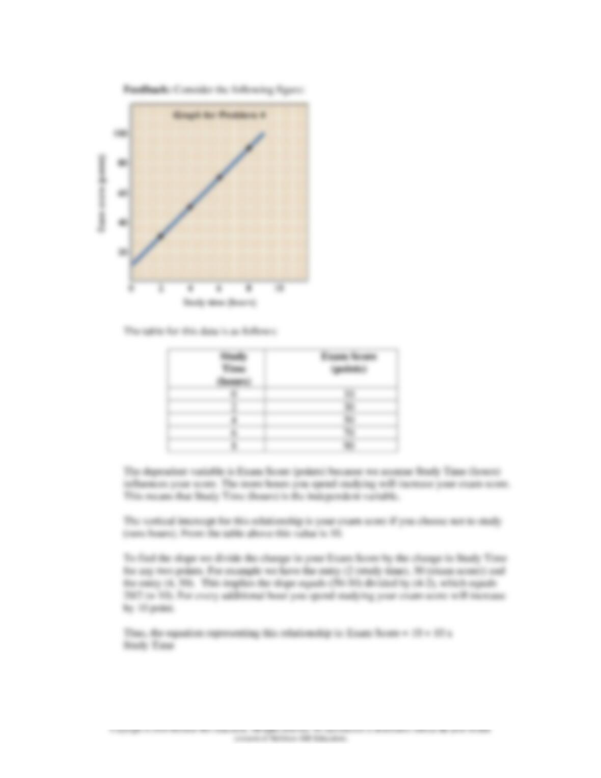
4. Construct a table from the data shown on the graph below. Which is the dependent variable
and which the independent variable? Summarize the data in equation form. LO8
Answer:
Study Time (hours)
Exam Score (points)
0
10
2
30
4
50
6
70
8
90
The dependent variable is Exam Score (points); Study Time (hours) is the
independent variable. Thus, the equation representing this relationship is: Exam
Score = 10 + 10 x Study Time.
Chapter 01 Appendix
1A–13
Copyright © 2018 McGraw-Hill Education. All rights reserved. No reproduction or distribution without the prior written
consent of McGraw-Hill Education.
Feedback: Consider the following figure:
The table for this data is as follows:
Study
Time
(hours)
Exam Score
(points)
0
10
2
30
4
50
6
70
8
90
The dependent variable is Exam Score (points) because we assume Study Time (hours)
influences your score. The more hours you spend studying will increase your exam score.
This means that Study Time (hours) is the independent variable.
The vertical intercept for this relationship is your exam score if you choose not to study
(zero hours). From the table above this value is 10.
To find the slope we divide the change in your Exam Score by the change in Study Time
for any two points. For example we have the entry (2 (study time), 30 (exam score)) and
the entry (4, 50). This implies the slope equals (50-30) divided by (4-2), which equals
20/2 (= 10). For every additional hour you spend studying your exam score will increase
by 10 point.
Thus, the equation representing this relationship is: Exam Score = 10 + 10 x
Study Time
1A–14
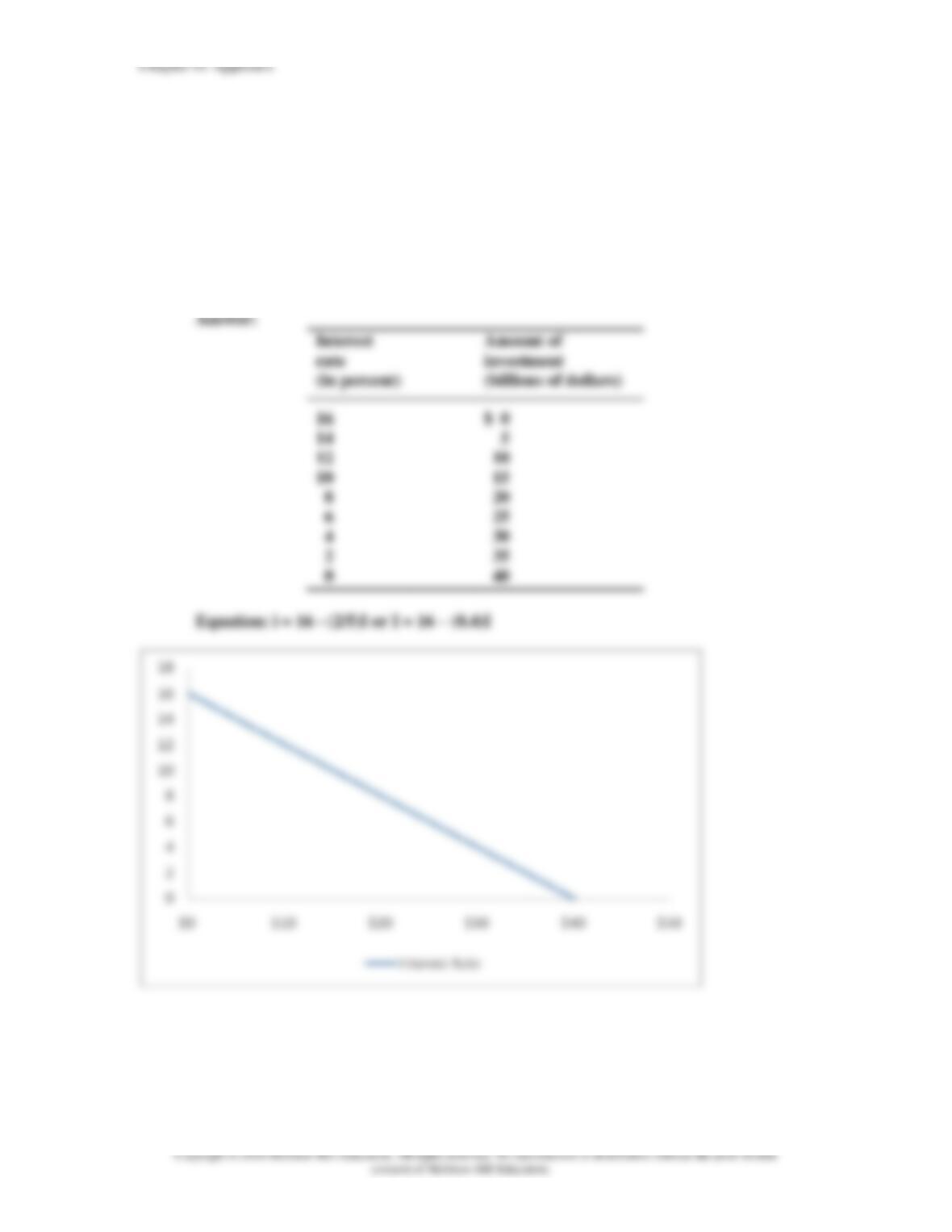
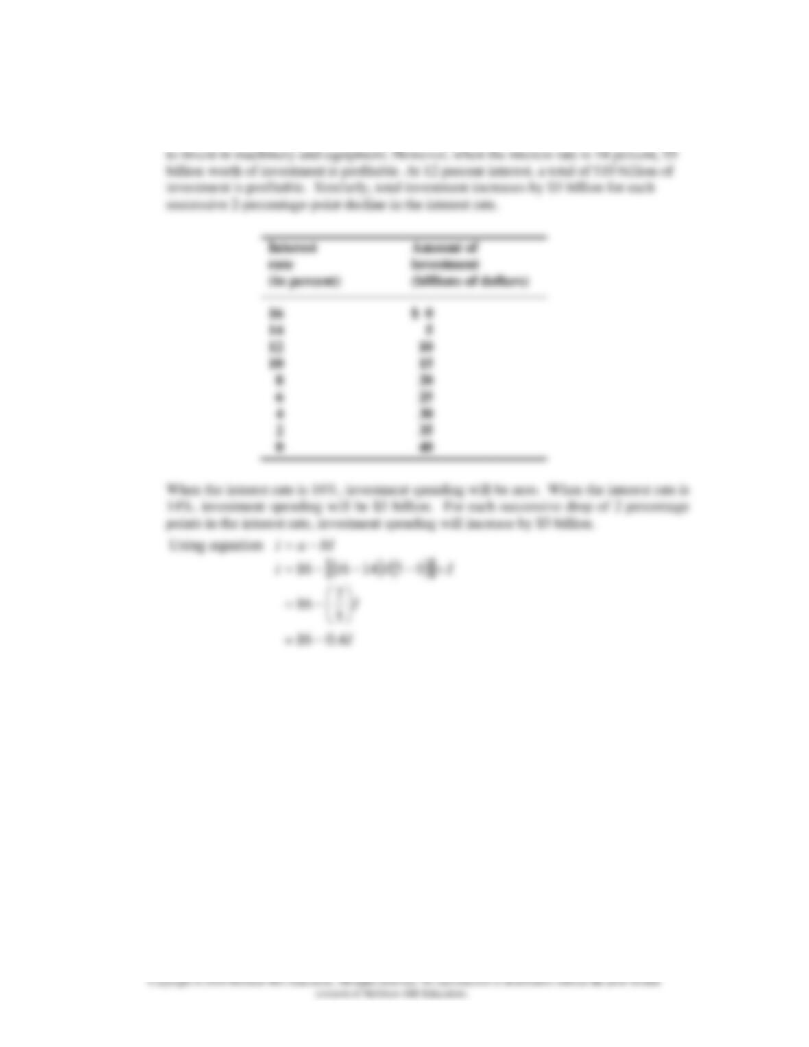
5. Suppose that when the interest rate on loans is 16 percent, businesses find it unprofitable to
invest in machinery and equipment. However, when the interest rate is 14 percent, $5 billion
worth of investment is profitable. At 12 percent interest, a total of $10 billion of investment is
profitable. Similarly, total investment increases by $5 billion for each successive 2-percentage-
point decline in the interest rate. Describe the relevant relationship between the interest rate and
investment in a table, on a graph, and as an equation. Put the interest rate on the vertical axis and
investment on the horizontal axis. In your equation use the form i = a + bI , where i is the interest
rate, a is the vertical intercept, b is the slope of the line (which is negative), and I is the level of
investment. LO8
Answer:
Interest
rate
(in percent)
Amount of
investment
(billions of dollars)
16
14
12
10
8
6
4
2
0
$ 0
5
10
15
20
25
30
35
40
Equation: i = 16 – (2/5)I or I = 16 – (0.4)I
Chapter 01 Appendix
1A–15
Feedback: Consider the following data as an example:
Suppose that when the interest rate on loans is 16 percent, businesses find it unprofitable
I
I
4.016
5
16
−=
−=
Chapter 01 Appendix
1A–16
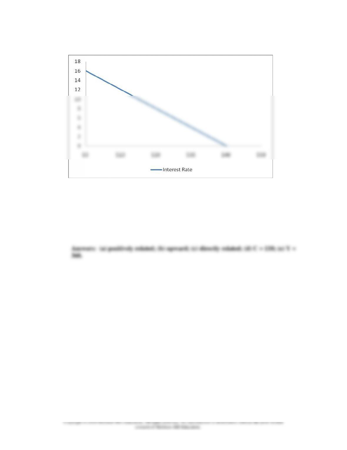
Graphically we have the following relationship.
6. Suppose that C = a + bY , where C = consumption, a = consumption at zero income, b = slope,
and Y = income. LO8
a. Are C and Y positively related or are they negatively related?
b. If graphed, would the curve for this equation slope upward or slope downward?
c. Are the variables C and Y inversely related or directly related?
d. What is the value of C if a = 10, b = .50, and Y = 200?
e. What is the value of Y if C = 100, a = 10, and b = .25?
Chapter 01 Appendix
1A–17
Feedback:
(a) C and Y are positively related because the slope, b, is positive by assumption. As
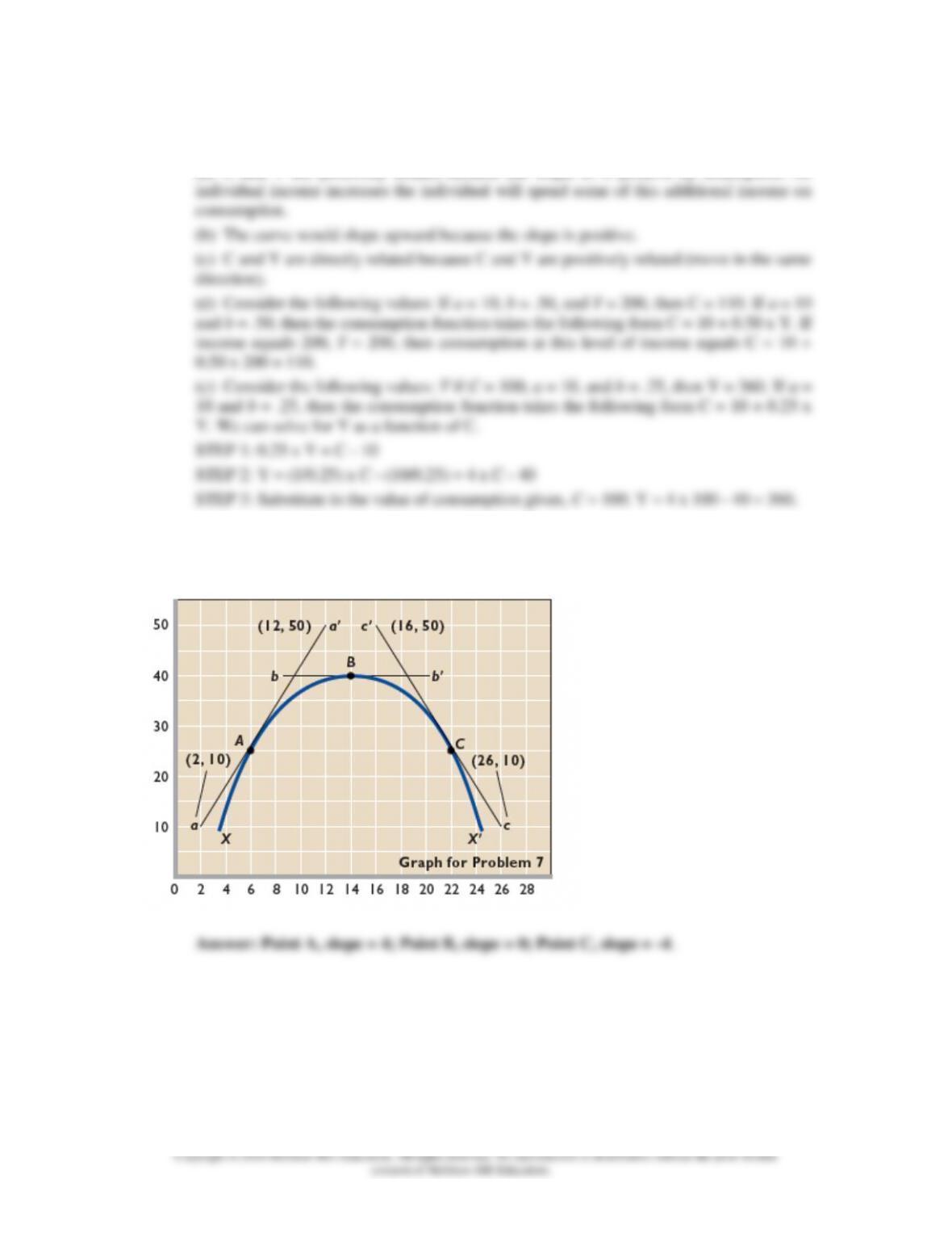
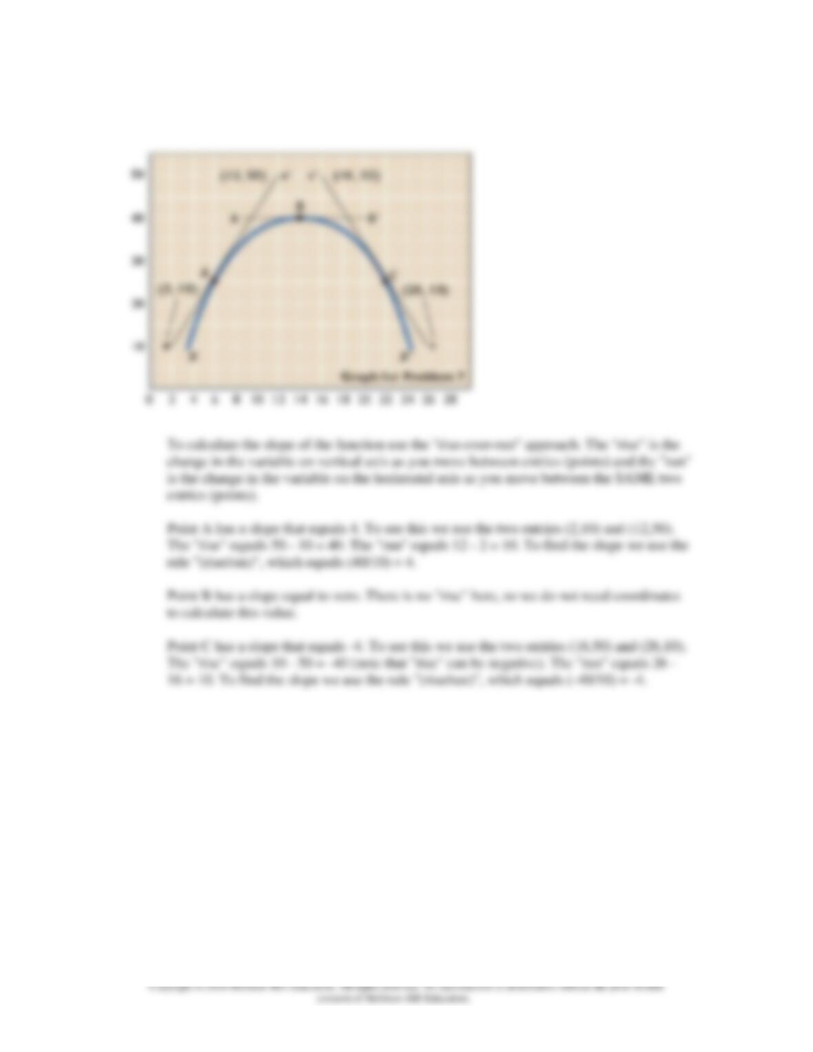
7. The accompanying graph shows curve XX’ and tangents at points A, B, and C. Calculate the
slope of the curve at these three points. LO8
Chapter 01 Appendix
1A–18
Feedback: Consider the following figure as an example:
1A–19
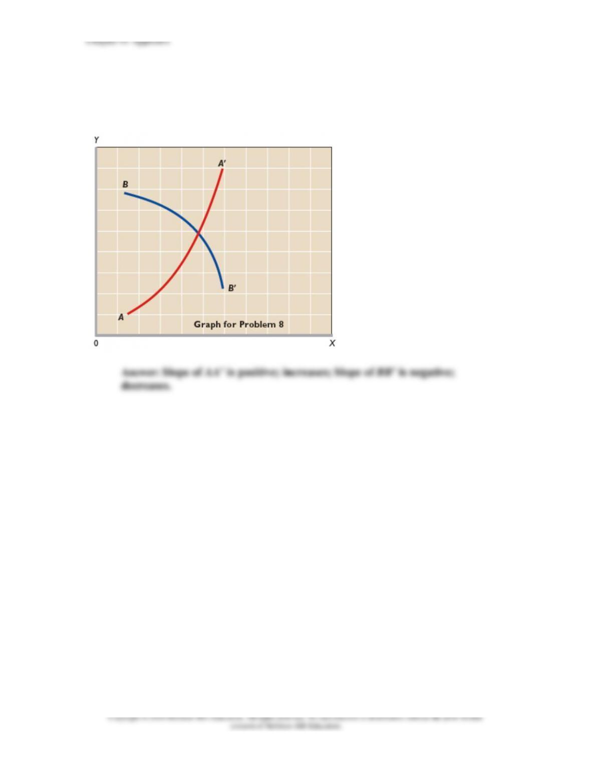
8. In the accompanying graph, is the slope of curve AA’ positive or negative? Does the slope
increase or decrease as we move along the curve from A to A’? Answer the same two questions
for curve BB’.
Chapter 01 Appendix
1A–20
Copyright © 2018 McGraw-Hill Education. All rights reserved. No reproduction or distribution without the prior written
consent of McGraw-Hill Education.
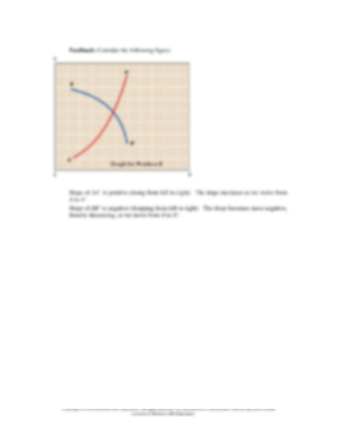
Feedback: Consider the following figure:
Slope of AA’ is positive (rising from left to right). The slope increases as we move from
A to A’.
Slope of BB’ is negative (dropping from left to right). The slope becomes more negative,
thereby decreasing, as we move from B to B’.