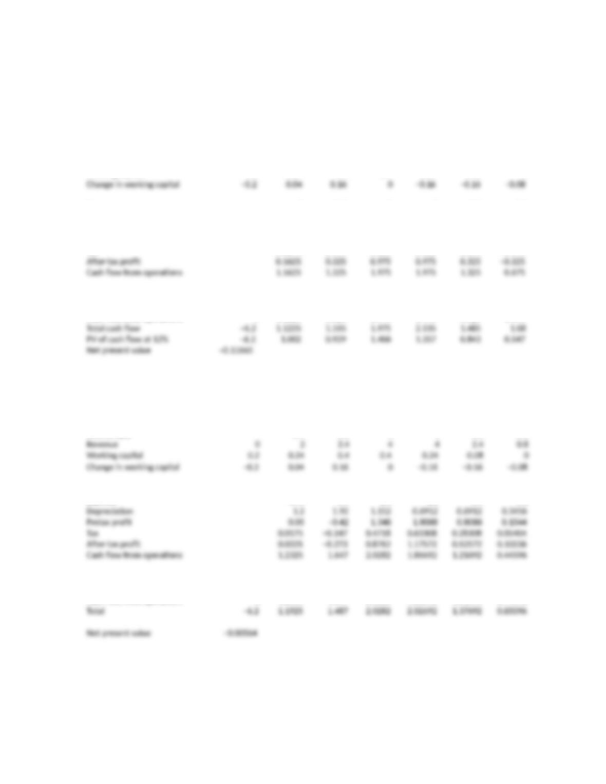
Year 0 1 2 3 4 5 6
Sales (traps) 0.5 0.6 1 1 0.6 0.2
Revenue 0 2 2.4 4 4 2.4 0.8
Working capital 0.2 0.24 0.4 0.4 0.24 0.08 0
Revenues 2 2.4 4 4 2.4 0.8
Expense 0.75 0.9 1.5 1.5 0.9 0.3
depreciation 1 1 1 1 1 1
Pretax profit 0.25 0.5 1.5 1.5 0.5 –0.5
Tax 0.0875 0.175 0.525 0.525 0.175 –0.175
Cash 0ow: capital invest. –6 0.325
Cash 0ow from WC –0.2 –0.04 –0.16 0 0.16 0.16 0.08
Cash 0ow from operation 0 1.1625 1.325 1.975 1.975 1.325 0.675
Year 0 1 2 3 4 5 6
Sales (traps) 0.5 0.6 1 1 0.6 0.2
Revenues 2 2.4 4 4 2.4 0.8
Expense 0.75 0.9 1.5 1.5 0.9 0.3
Cash 0ow: capital invest. –6 0.325
Cash 0ow from WC –0.2 –0.04 –0.16 0 0.16 0.16 0.08
Cash 0ow from operation 0 1.2325 1.647 2.0282 1.86692 1.21692 0.44596
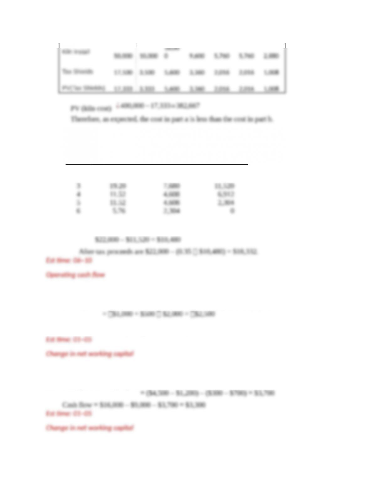
1. All cash flows are in millions of dollars. Sales price of machinery in year 6 is shown on
an after-tax basis as a positive cash flow on the capital investment line.
a.
…
b. ….
….
Using the 5-year MACRS schedule, the net present value increases by $111,010 (=
116,650 – 5,640).
Est time: 11–15
9–
Copyright © 2018 McGraw-Hill Education. All rights reserved. No reproduction or distribution without the prior written consent of
McGraw-Hill Education.
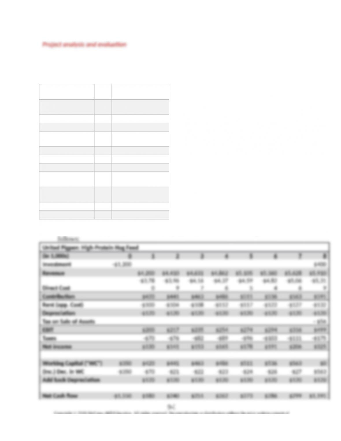
2. The assumptions for the Pigpen project are laid out in the table below:
Investment $1.
2
million
Revenue $4.
2
million
Rev growth 5% per annum
Manufacture costs 90% of sales
Rent (opp. Cost) $10
0
thousand
Rent Growth 4% per annum
Dep’n Life 10 years
Tax Rate 35% marginal
Plant Salet=8 $40
0
thousand
WC investment $35
0
thousand
WC ongoing 10% of sales
Cost of Capital 12%
Using these assumptions, we can schedule project cash flows across the 8 year horizon as
Copyright © 2018 McGraw-Hill Education. All rights reserved. No reproduction or distribution without the prior written consent of
McGraw-Hill Education.
Est time: 11–15
Project analysis and evaluation
3. While depreciation is a noncash expense, it has an impact on net cash flow because of its
impact on taxes. Every dollar of depreciation expense reduces taxable income by one
4. Depreciation expense per year = $40/5 = $8 million
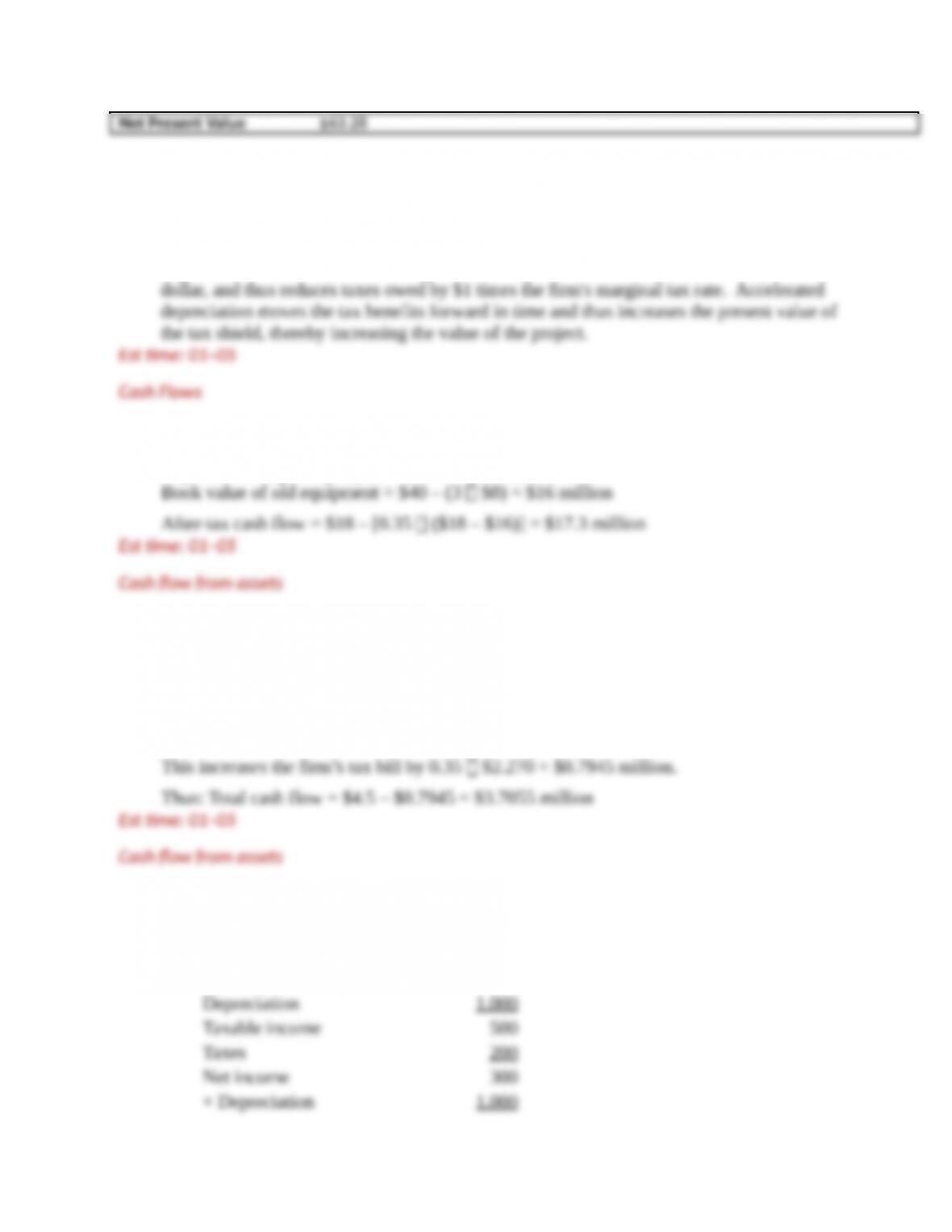
5. Using the 7-year MACRS depreciation schedule, after 5 years the machinery will be
written down to 22.30% of its original value: 0.2230 $10 million = $2.230 million
If the machinery is sold for $4.5 million, the sale generates a taxable gain of $2.270
million.
6. a. All values should be interpreted as incremental results from making the purchase.
Earnings before depreciation $1,500
9–
Copyright © 2018 McGraw-Hill Education. All rights reserved. No reproduction or distribution without the prior written consent of
McGraw-Hill Education.
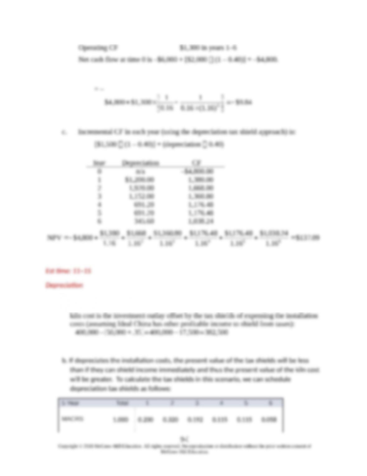
b. NPV = –$4,800 + [$1,300 annuity factor (16%, 6 years)]
7. a. If Ideal China expenses the installation costs immediately, then the present value of the
16,00
8. a.
Year MACRS (%) Depreciation Book Value
(end of year)
1
20.00
$ 8,000
$32,000
2 32.00 12,800 19,200
b. If the machine is sold for $22,000 after 3 years, sales price exceeds book value by:
9. a. NWC = accounts receivable + inventory accounts payable
b. Cash flow = $36,000 $24,000 + $2,500 = $14,500
10. Change in working capital = accounts receivable – accounts payable
9–
Copyright © 2018 McGraw-Hill Education. All rights reserved. No reproduction or distribution without the prior written consent of
McGraw-Hill Education.
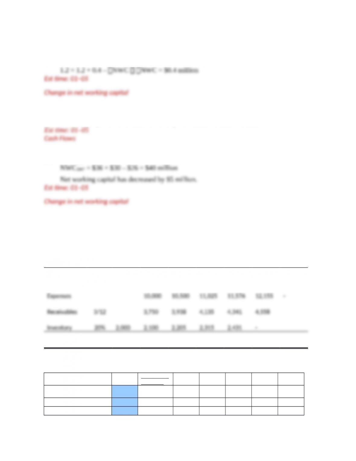
11. Cash flow = net income + depreciation – increase in NWC
12. Cash flow = profit – increase in inventory = $10,000 – $1,000 = $9,000
13. NWC2016 = $32 + $25 – $12 = $45 million
14.
a. Lower. The NPV decreases from $4,223 to $3,458. See the valuation used in part c.
b.
0 1 2 3 4 5 6
Revenue
15,000
15,750
16,538
17,364
18,233
–
Working Capital
2,000
5,850
6,143
6,450
6,772
4,558
A. Inputs
Spreadshe
et Name
Initial Investment 10,000
Investmen
t
Salvage value 2,000 Salvage
Initial revenue 15,000 Initial_rev
9–
Copyright © 2018 McGraw-Hill Education. All rights reserved. No reproduction or distribution without the prior written consent of
McGraw-Hill Education.
Initial expenses 10,000 Intial_exp
Inflation rate 0.05 Inflation
Discount rate 0.12 Disc_rate
Acct receiv. as % of
sales 1/4 A_R
Inven. as % of
expenses 0.2 Inv_pct
Tax rate 0.35 Tax_rate
Year: 0 1 2 3 4 5 6
B. Fixed assets
Investments in fixed
assets 10,000
C. Operating cash
ow
Revenues 15,000 15,750 16,538 17,364 18,233
Expenses 10,000 10,500 11,025 11,576 12,155
Depreciation 2,000 2,000 2,000 2,000 2,000
Pretax pro)t 3,000 3,250 3,513 3,788 4,078
Tax 1,050 1,138 1,229 1,326 1,427
profit after tax 1,950 2,113 2,283 2,462 2,650
Cash flow from
operations 3,950 4,113 4,283 4,462 4,650
D. Working capital
E. Project valuation
-12,00
Net present value 3,458
Est time: 06–10
Net Present Value
9–
Copyright © 2018 McGraw-Hill Education. All rights reserved. No reproduction or distribution without the prior written consent of
McGraw-Hill Education.
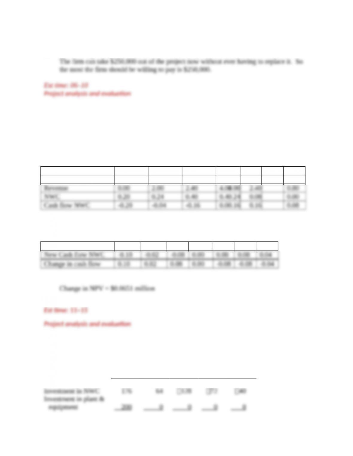
15. If the savings are permanent, then the inventory system is worth $250,000 to the firm.
16. Some values below may show as rounded for display purposes, though unrounded
numbers should be used for actual calculations.
All cash flows are in millions of dollars. Sales price of machinery in year 6 is shown on an
after-tax basis as a positive cash flow on the capital investment line.
Year 0 1 2 3 6
Sales units 0.00 0.50 0.60 1.001.00 0.60 0.20
If working capital requirements were only one-half of the expected amount, then the
working capital cash-flow forecasts would change as follows:
New NWC 0.10 0.12 0.20 0.20 0.12 0.04 0.00
17.
All figures in thousands
01234
Net working capital
$176
$240
$112
$40
$ 0
9–
Copyright © 2018 McGraw-Hill Education. All rights reserved. No reproduction or distribution without the prior written consent of
McGraw-Hill Education.
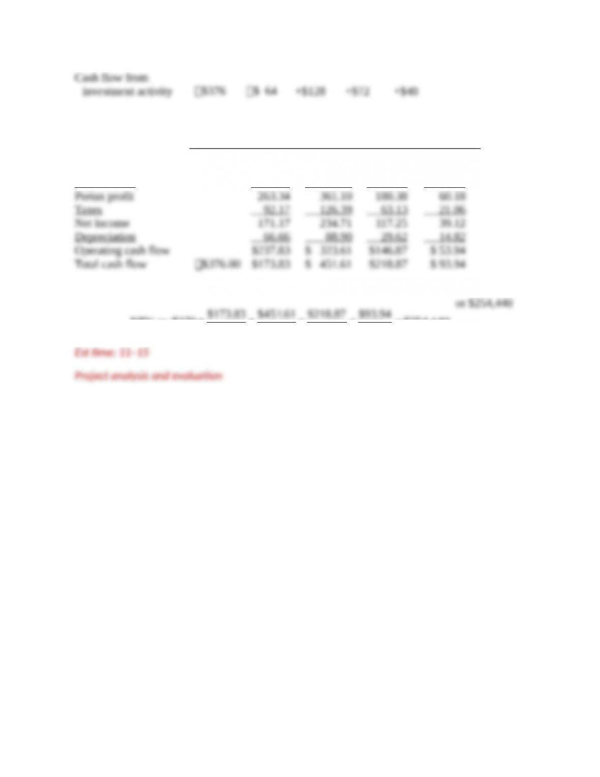
All figures in thousands
0 1 2 3 4
Revenue
$880.00
$1,200.00
$560.00
$200.00
Cost 550.00 750.00 350.00 125.00
Depreciation 66.66 88.90 29.62 14.82