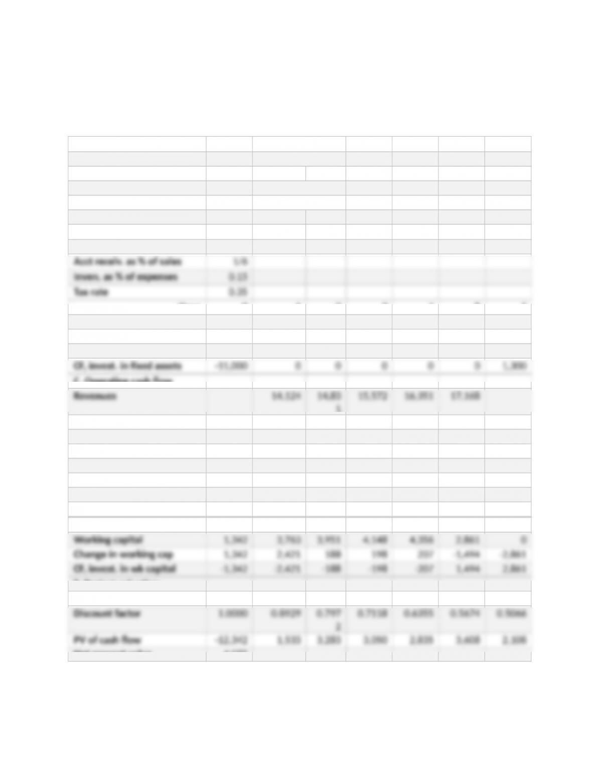
a. Use goal seek to isolate profit after tax as the dependent variable relating to initial
revenue. The level of initial revenue in the base case was $15,000,000, which
produced accounting profits of $11,458,000 across the five project years. Adjusting
the spreadsheet to the scenario presented here, initial revenue can fall to $14,124,000
before accounting profits fall below $11,458,000:
A. Inputs
Initial investment 11,000
Salvage value 2,000
Initial revenue 14,124
Initial fixed expenses 4,000
Expenses % of Revenue 0.35
Inflation rate 0.05
Discount rate 0.12
Year: 0 1 2 3 4 5 6
B. Capital investment
Investment in fixed assets 11,000
Sales of fixed assets 1,300
C. Operating cash flow
1
Variable expenses 4,944 5,191 5,450 5,723 6,009
Fixed expenses 4,000 4,200 4,410 4,631 4,862
Depreciation 2,200 2,200 2,200 2,200 2,200
Pretax profit 2,981 3,240 3,512 3,798 4,097
Tax 1,043 1,134 1,229 1,329 1,434
Profit a3er tax 1,938 2,106 2,283 2,468 2,663
Operating cash flow 4,138 4,306 4,483 4,668 4,863
D. Changes in working capital
E. Project valuation
Total project cash flow -12,342 1,716 4,118 4,285 4,461 6,358 4,161
Net present value 4,075
b. Use goal seek to isolate net present value as the dependent variable relating to initial
revenue. The level of initial revenue in the base case was $15,000,000, which
10-‘
Copyright © 2018 McGraw-Hill Education. All rights reserved. No reproduction or distribution without the prior written consent of
McGraw-Hill Education.
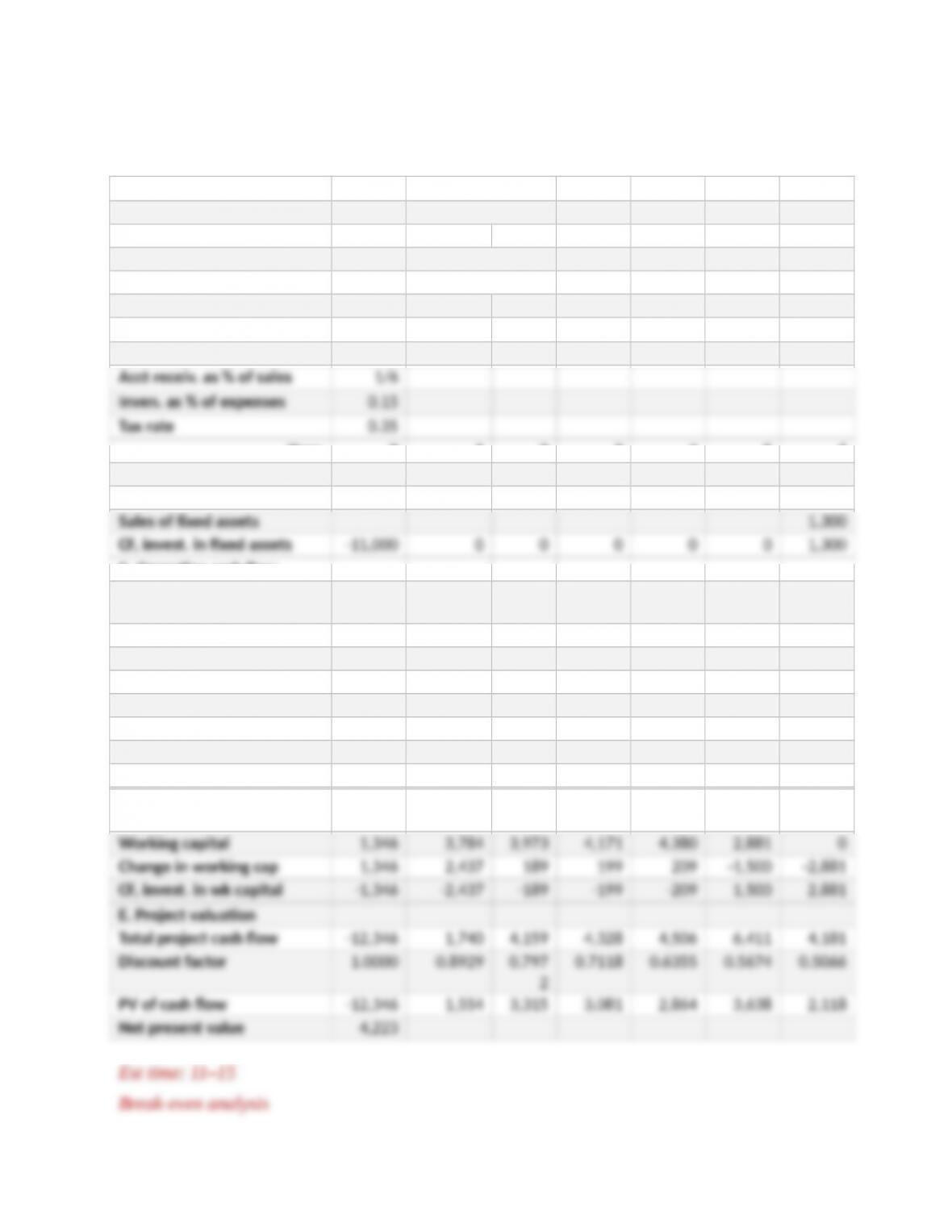
produced net present value of $4,223,000. Adjusting the spreadsheet to the scenario
presented here, initial revenue can fall to $14,219,000 before net present value falls
below $4,223,000:
A. Inputs
Initial investment 11,000
Salvage value 2,000
Initial revenue 14,219
Initial fixed expenses 4,000
Expenses % of Revenue 0.35
Inflation rate 0.05
Discount rate 0.12
Year: 0 1 2 3 4 5 6
B. Capital investment
Investment in fixed assets 11,000
C. Operating cash flow
Revenues 14,219 14,93
0
15,676 16,460 17,283
Variable expenses 4,977 5,225 5,487 5,761 6,049
Fixed expenses 4,000 4,200 4,410 4,631 4,862
Depreciation 2,200 2,200 2,200 2,200 2,200
Pretax profit 3,042 3,304 3,580 3,869 4,172
Tax 1,065 1,157 1,253 1,354 1,460
Profit a3er tax 1,978 2,148 2,327 2,515 2,712
Operating cash flow 4,178 4,348 4,527 4,715 4,912
D. Changes in working
capital
10-‘
Copyright © 2018 McGraw-Hill Education. All rights reserved. No reproduction or distribution without the prior written consent of
McGraw-Hill Education.
1. NPV will be negative. We’ve shown in the previous problem that the accounting
2. Percentage change in profits = percentage change in sales DOL.
3. DOL =
fixed costs (including depreciation)
1profits
+
a. Profit = revenues – variable costs – fixed costs – depreciation
4. DOL =
fixed costs (including depreciation)
1profits
+
10-‘
Copyright © 2018 McGraw-Hill Education. All rights reserved. No reproduction or distribution without the prior written consent of
McGraw-Hill Education.
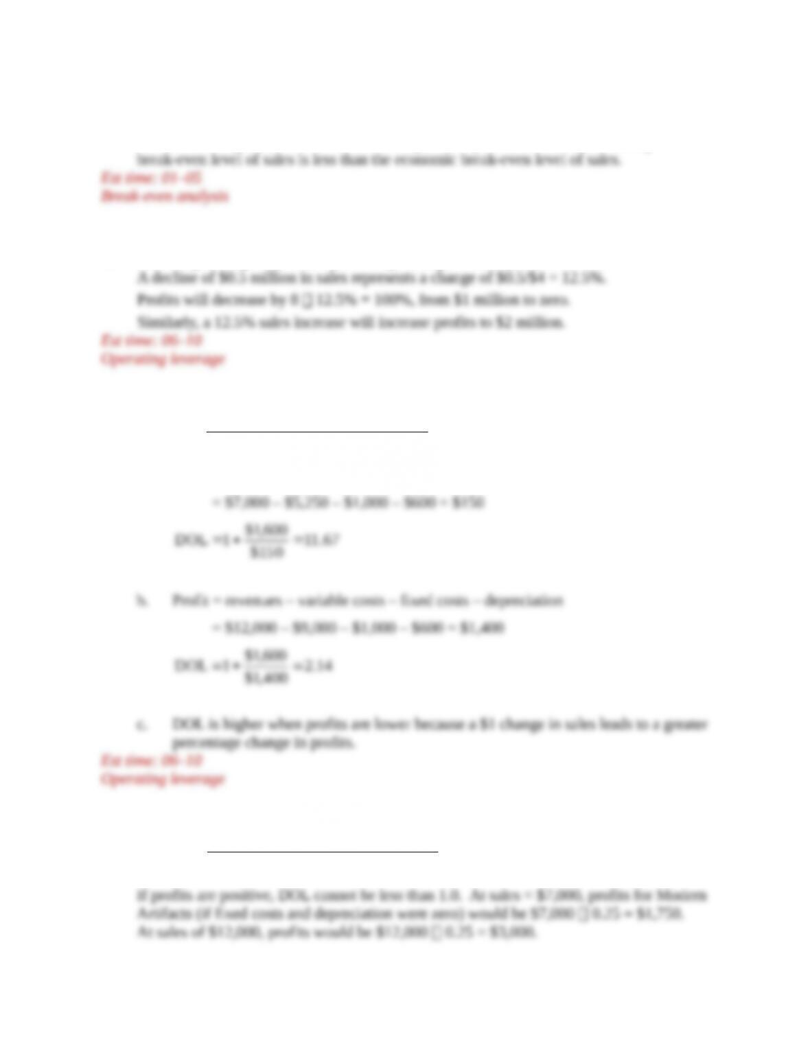
5. a. Pretax profits currently equal:
Revenue – variable costs – fixed costs – depreciation
b. DOL =
4
500$
500,1$
1
ofitspr
on)depreciati (including costs fixed
1
6.
a The option to delay expansion is a Timing Option because the decision to expand is not
7. We compare expected NPV with and without testing. If the field is large, then:
10-‘
Copyright © 2018 McGraw-Hill Education. All rights reserved. No reproduction or distribution without the prior written consent of
McGraw-Hill Education.
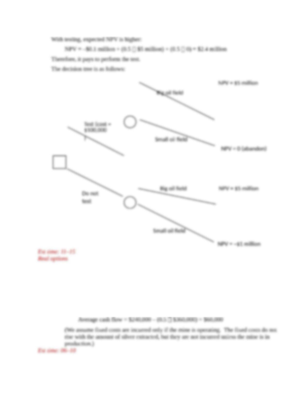
24. a. Average annual expenses = (10,000 $32) + $40,000 = $360,000
Average annual revenue = 10,000 (.5 × $24) + 10,000 (.5 × $48) = $360,000
Average cash flow = revenue – expenses = $360,000 – $360,000 = $0
b. If you can shut down the mine 50% of the time, CF in the low-price years will be zero. In
the remaining years:
10-‘
Copyright © 2018 McGraw-Hill Education. All rights reserved. No reproduction or distribution without the prior written consent of
McGraw-Hill Education.
Real options
25.
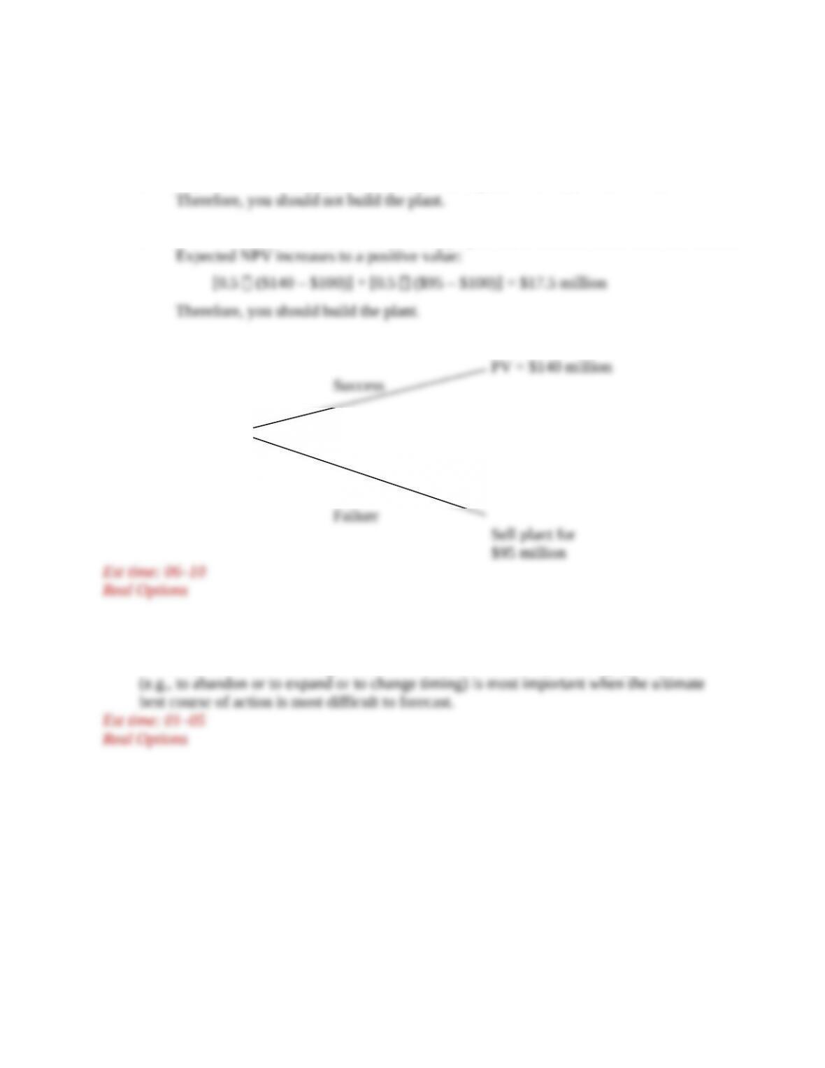
a. Expected NPV = [0.5 ($140 – $100)] + [0.5 ($50 – $100)] = –$5 million
b. Now the worst-case value of the installed project is $95 million rather than $50 million.
c.
Invest
$100 million
26. Options provide the ability to cut losses or to extend gains. You benefit from good
outcomes but can limit damage from bad outcomes. The ability to change your actions
10-‘
Copyright © 2018 McGraw-Hill Education. All rights reserved. No reproduction or distribution without the prior written consent of
McGraw-Hill Education.
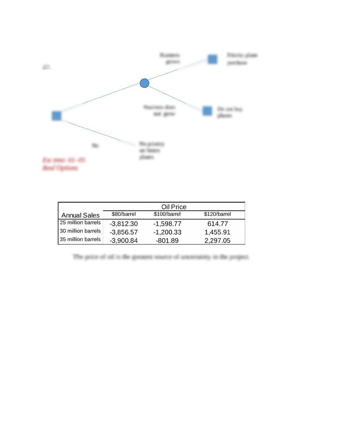
28. a.
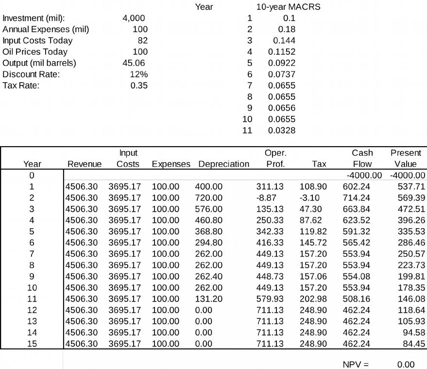
b. Given a $100 per barrel price, the annual level of sales necessary for an NPV break-even
is 45.00 million barrels. The value was found using Excel’s Goal Seek, shown below:
10-‘
Copyright © 2018 McGraw-Hill Education. All rights reserved. No reproduction or distribution without the prior written consent of
McGraw-Hill Education.
Decision to
buy option
10-‘
Copyright © 2018 McGraw-Hill Education. All rights reserved. No reproduction or distribution without the prior written consent of
McGraw-Hill Education.
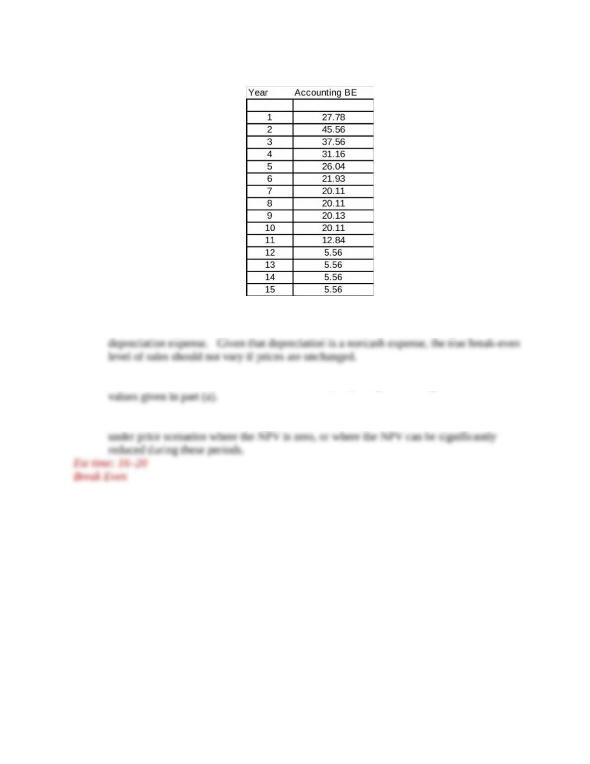
c.
The accounting break-even level of sales changes each year with the changes in
d. The NPV of –$1,200.33 million is found as an equally weighted average for all NPV
e. The facility may be worth building if the firm has the option to shut down the facilities
10-‘
Copyright © 2018 McGraw-Hill Education. All rights reserved. No reproduction or distribution without the prior written consent of
McGraw-Hill Education.