Solutions to Chapter 10
Project Analysis
1. Scenario analysis – Project NPV is recalculated by changing several inputs to new but
consistent values.
Real option – Opportunity to modify a project at a future date.
Sensitivity analysis – Analysis of how project NPV changes if different assumptions are
2.
False – Approval of the capital budget allows manager to go ahead with any project
included in the budget.
3.
True – Sensitivity analysis can be used to identify the variables most crucial to a project’s
success.
4.
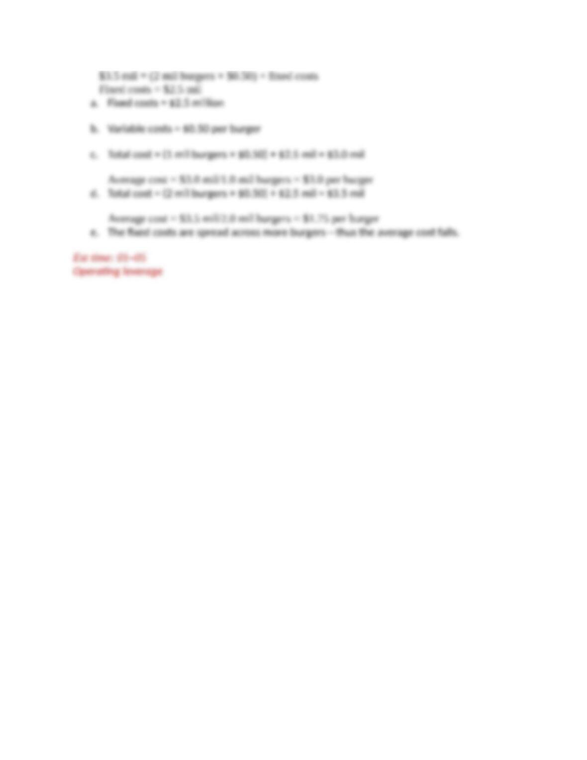
The extra 2 million burgers increase total costs by $1.0 million.
10-6
Copyright © 2018 McGraw-Hill Education. All rights reserved. No reproduction or distribution without the prior written consent of
McGraw-Hill Education.
5.
10-6
Copyright © 2018 McGraw-Hill Education. All rights reserved. No reproduction or distribution without the prior written consent of
McGraw-Hill Education.
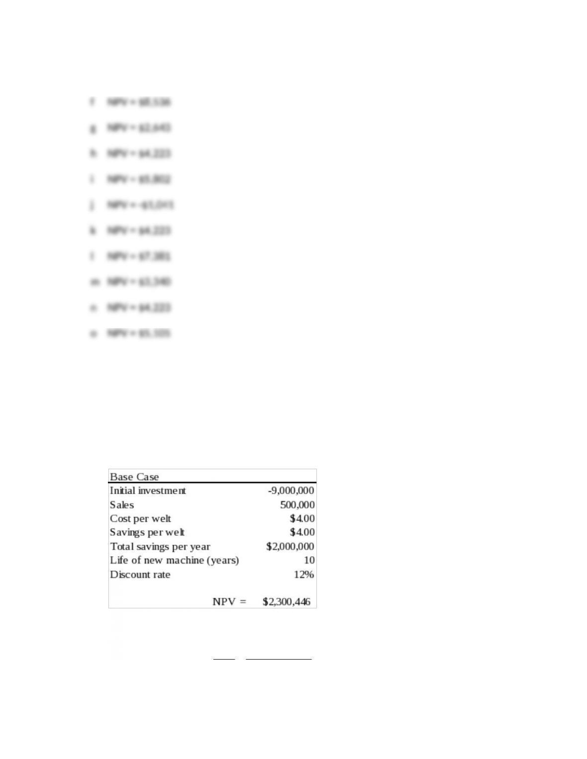
6. Use the student spreadsheet provided for Blooper’s to calculate NPVs (in thousands):
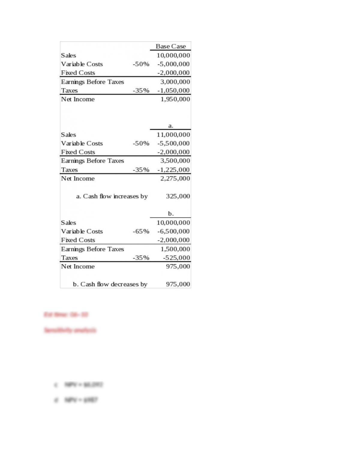
a NPV = $484
b NPV = $4,223
10-6
Copyright © 2018 McGraw-Hill Education. All rights reserved. No reproduction or distribution without the prior written consent of
McGraw-Hill Education.
e NPV = $4,223
Est time: 06–10
Sensitivity analysis
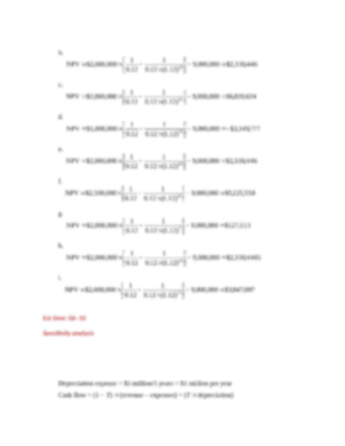
7.
a.
357,40$000,000,9
)12.1(0.12
1
0.12
1
$1,600,000NPV 10
10-6
Copyright © 2018 McGraw-Hill Education. All rights reserved. No reproduction or distribution without the prior written consent of
McGraw-Hill Education.
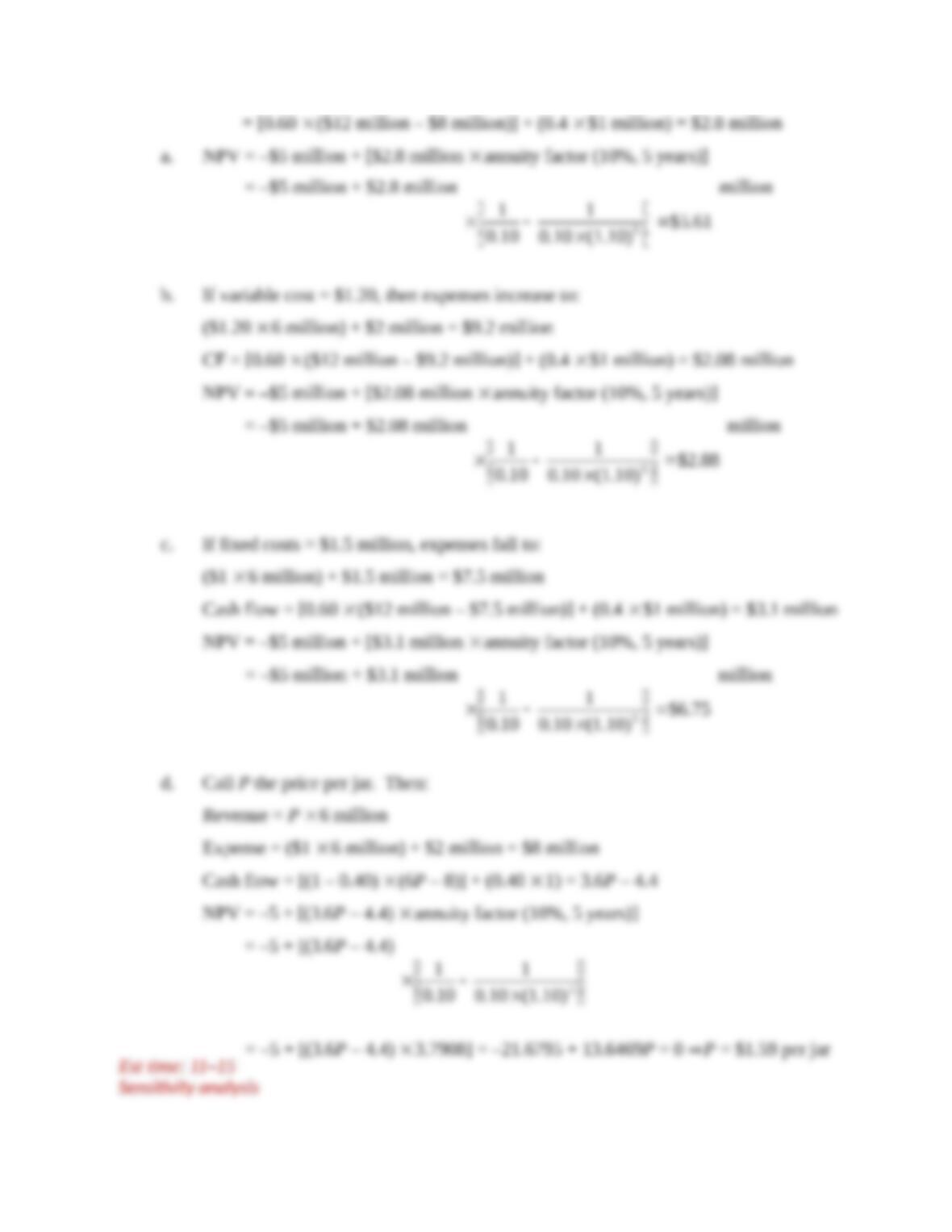
8. Revenue = price quantity = $2 6 million = $12 million
Expense = variable cost + fixed cost = ($1 6 million) + $2 million = $8 million
10-6
Copyright © 2018 McGraw-Hill Education. All rights reserved. No reproduction or distribution without the prior written consent of
McGraw-Hill Education.
10-6
Copyright © 2018 McGraw-Hill Education. All rights reserved. No reproduction or distribution without the prior written consent of
McGraw-Hill Education.
9.
Most Likely Best Case Worst Case
Price
$50
$55
$45
Variable cost $30 $27 $33
Fixed cost $300,000 $270,000 $330,000
Sales 30,000 units 33,000 units 27,000 units
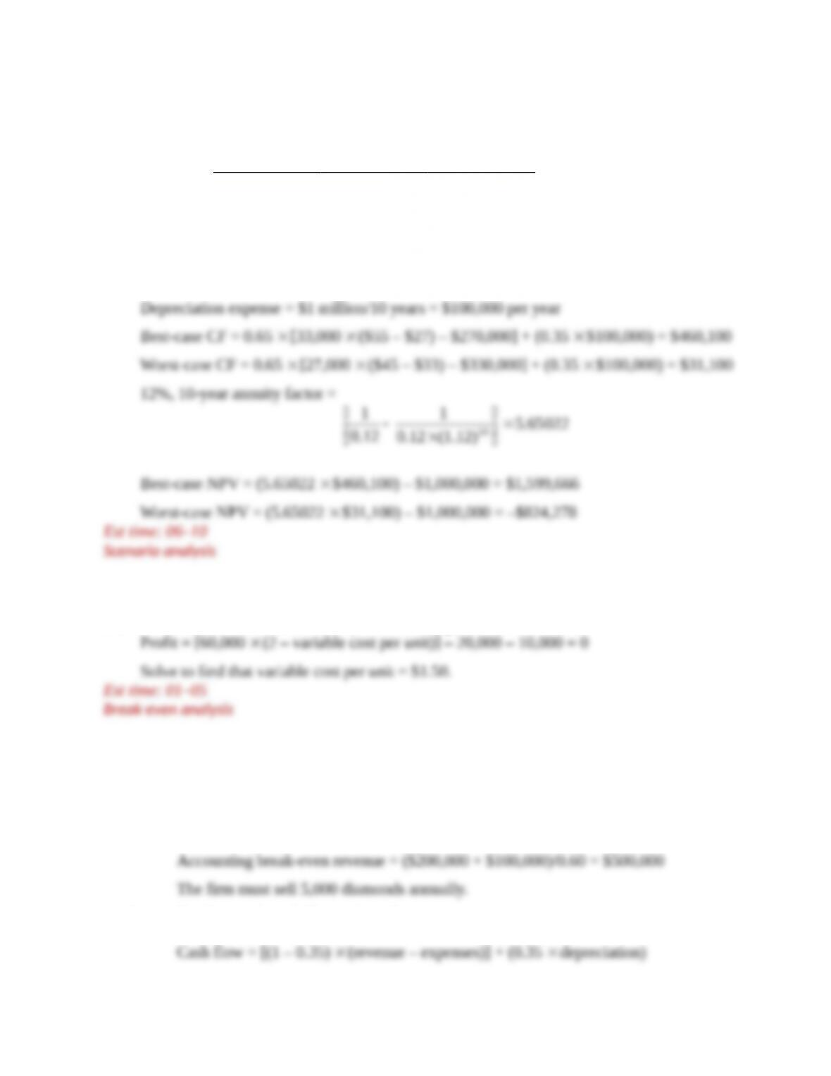
Cash flow = [(1 – T) (revenue – cash expenses)] + (T depreciation)
10. At the break-even level of sales (60,000 units) profit would be zero:
11.
a. Each dollar of sales generates $0.60 of pretax profit. depreciation expense is $100,000
per year, and fixed costs are $200,000. Therefore:
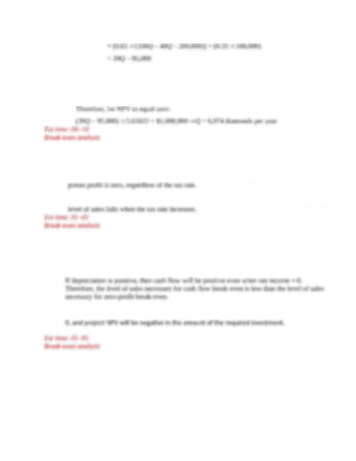
b. Let Q = the number of diamonds sold.
10-6
Copyright © 2018 McGraw-Hill Education. All rights reserved. No reproduction or distribution without the prior written consent of
McGraw-Hill Education.
12%, 10-year annuity factor =
65022.5
(1.12)0.12
1
0.12
1
10
12.
a. The accounting break-even point would be unaffected since taxes paid are zero when
b. The NPV break-even point would increase since the after-tax cash flow corresponding to any
13.
a Cash 9ow = net income + depreciation
b. If cash 9ow = 0 for the entire life of the project, then the present value of cash 9ows =
14. a., b.
10-6
Copyright © 2018 McGraw-Hill Education. All rights reserved. No reproduction or distribution without the prior written consent of
McGraw-Hill Education.
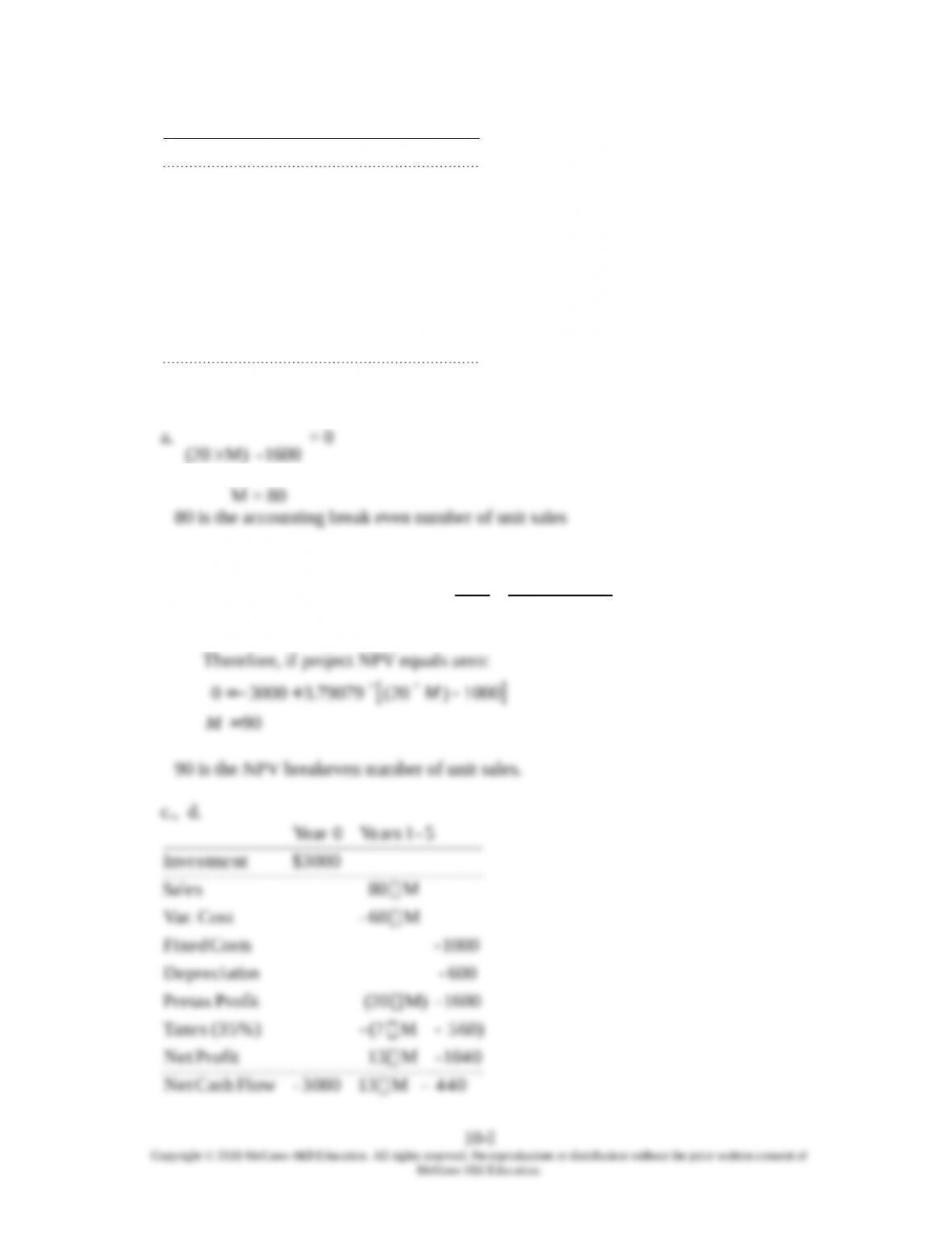
1000 – M) (20 3000-FlowCash Net
1600 – M) (20 ProfitNet
0(0%) Taxes
1600 – M) (20 ProfitPretax
600- onDepreciati
1000- Costs Fixed
M 60-Cost Var.
M 80 Sales
$3000Investment
5-1 Years0Year
a.
1600 – M) (20
= 0
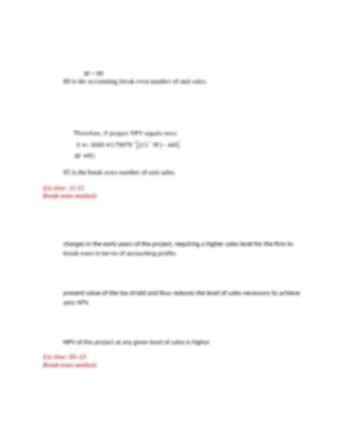
M = 80
80 is the accounting break even number of unit sales
b. The 10%, 5-year annuity factor is:
79079.3
(1.10)0.10
1
0.10
1
5
d. The 10%, 5-year annuity factor is:
79079.3
(1.10)0.10
1
0.10
1
5
15.
a accounting break-even level of sales increases. MACRS results in higher depreciation
b. NPV break-even level of sales decreases. The accelerated depreciation increases the
c. MACRS makes the project more aBrac5ve. The PV of the tax shield is higher, so the
16.
10-6
Copyright © 2018 McGraw-Hill Education. All rights reserved. No reproduction or distribution without the prior written consent of
McGraw-Hill Education.
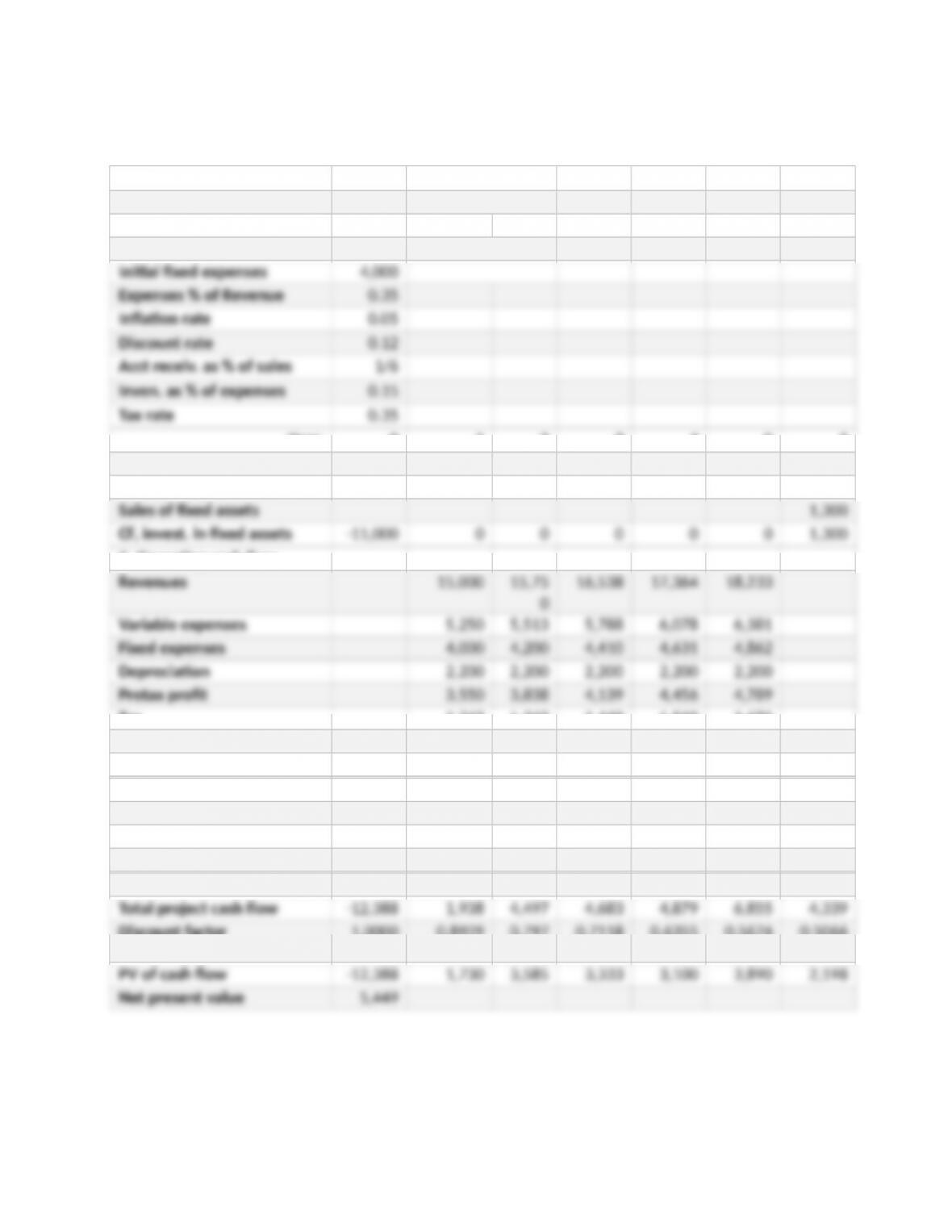
a. The analysis under the new scenario is as follows:
A. Inputs
Initial investment 11,000
Salvage value 2,000
Initial revenue 15,000
Year: 0 1 2 3 4 5 6
B. Capital investment
Investment in fixed assets 11,000
C. Operating cash ow
Tax 1,243 1,343 1,449 1,560 1,676
Profit a3er tax 2,308 2,494 2,691 2,897 3,113
Operating cash ow 4,508 4,694 4,891 5,097 5,313
D. Changes in working capital
Working capital 1,388 3,957 4,155 4,362 4,581 3,039 0
Change in working cap 1,388 2,569 198 208 218 -1,542 -3,039
CF, invest. in wk capital -1,388 -2,569 -198 -208 -218 1,542 3,039
E. Project valuation
Discount factor 1.0000 0.8929 0.797
2
0.7118 0.6355 0.5674 0.5066
10-6
Copyright © 2018 McGraw-Hill Education. All rights reserved. No reproduction or distribution without the prior written consent of
McGraw-Hill Education.