Chapter 11
Diversification and Risky Asset Allocation
Concept Questions
1. Based on market history, the average annual standard deviation of return for a single, randomly
2. If the returns on two stocks are highly correlated, they have a strong tendency to move up and down
6. The common answer might be that over time volatility cancels out; however, this is incorrect and is
7. An investment with high volatility could actually reduce the risk of the overall portfolio if its
8. The importance of the minimum variance portfolio is that it determines the lower bound of the
10. If two assets have zero correlation and the same standard deviation, then evaluating the general
Copyright © 2018 McGraw-Hill Education. All rights reserved. No reproduction or distribution without the prior written consent of McGraw-Hill
Education.
Solutions to Questions and Problems
NOTE: All end of chapter problems were solved using a spreadsheet. Many problems require multiple
steps. Due to space and readability constraints, when these intermediate steps are included in this
solutions manual, rounding may appear to have occurred. However, the final answer for each problem is
found without rounding during any step in the problem.
Core Questions
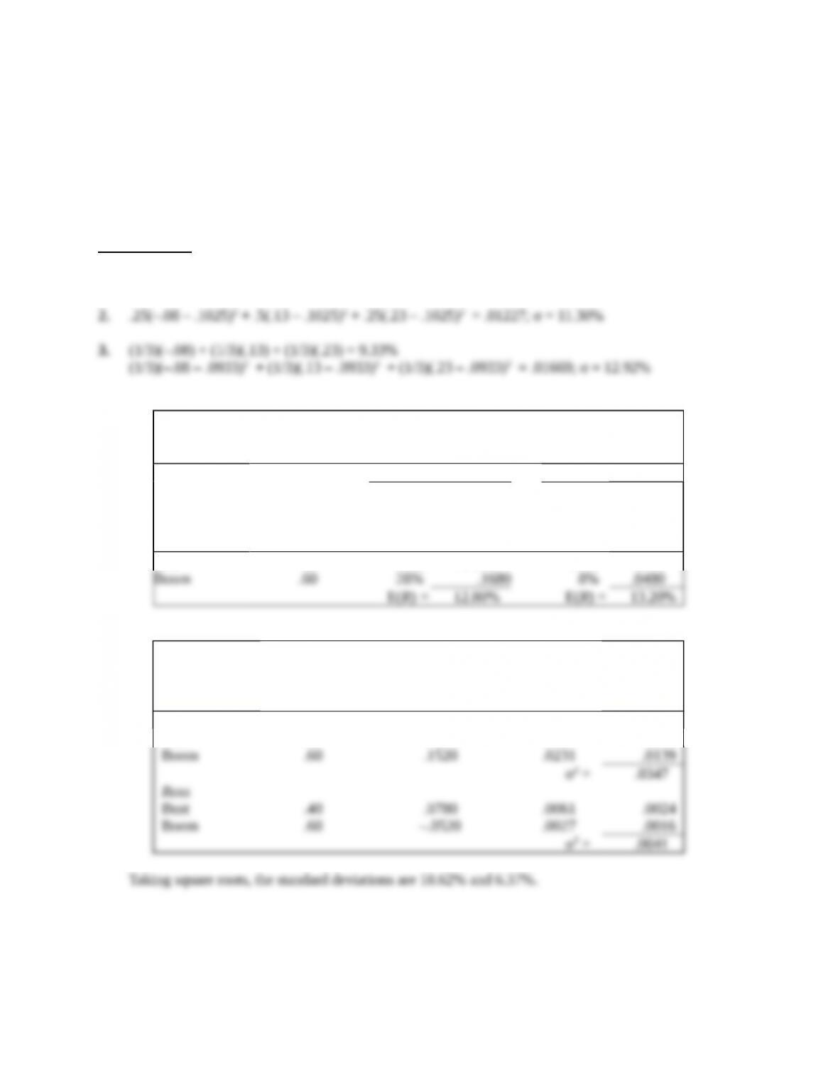
1. .25(–.08) + .5(.13) + .25(.23) = 10.25%
4.
Calculating Expected Returns
Roll Ross
(1)
State of
Economy
(2)
Probability of
State of
Economy
(3)
Return if
State
Occurs
(4)
Product
(2) × (3)
(5)
Return if
State
Occurs
(6)
Product
(2) × (5)
Bust .40 –10% –.0400 21% .0840
5.
(1)
State
of Economy
(2)
Probability of
State of
Economy
(3)
Return Deviation
from Expected
Return
(4)
Squared
Return
Deviation
(5)
Product
(2) × (4)
Roll
Bust .40 –.2280 .0520 .0208
Copyright © 2018 McGraw-Hill Education. All rights reserved. No reproduction or distribution without the prior written consent of McGraw-Hill
Education.
6.
Expected Portfolio Return
(1)
State of
Economy
(2)
Probability of
State of
Economy
(3)
Portfolio Return if State Occurs
(4)
Product
(2) × (3)
7.
Calculating Portfolio Variance
(1)
State of
Economy
(2)
Probability of
State of Economy
(3)
Portfolio Return
if State Occurs
(4)
Squared Deviation from
Expected Return
(5)
Product
(2) × (4)
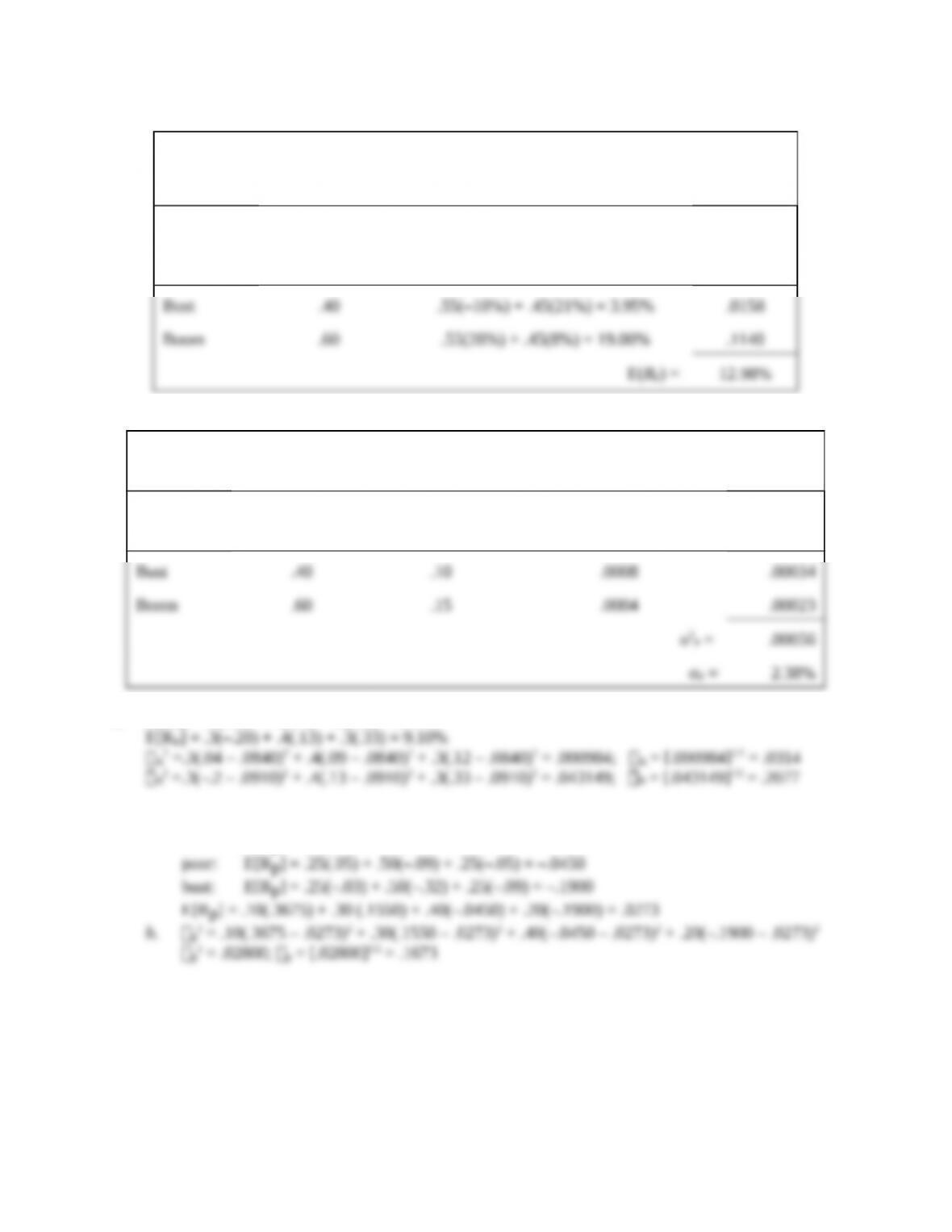
8. E[RA] = .3(.04) + .4(.09) + .3(.12) = 8.40%
9. a. boom: E[Rp] = .25(.18) + .50(.48) + .25(.33) = .3675
good: E[Rp] = .25(.11) + .50(.18) + .25(.15) = .1550
Copyright © 2018 McGraw-Hill Education. All rights reserved. No reproduction or distribution without the prior written consent of McGraw-Hill
Education.
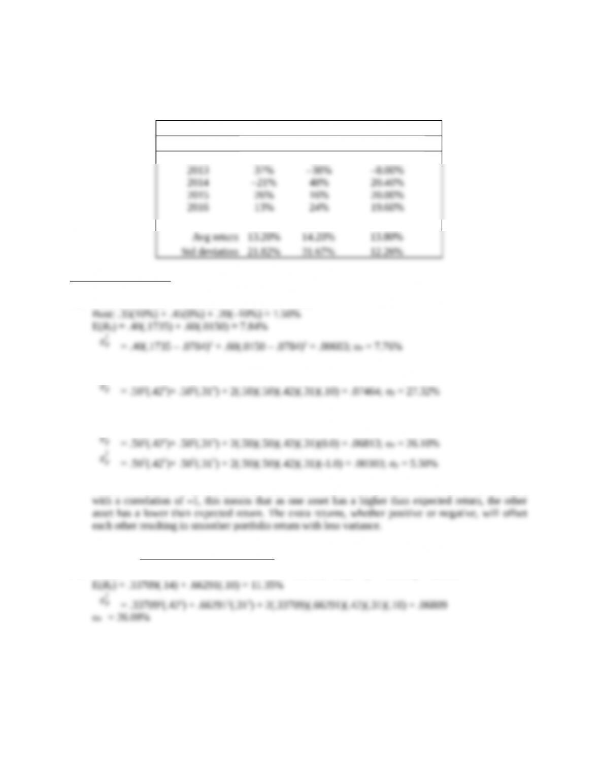
10. Notice that we have historical information here, so we calculate the sample average and sample
standard deviation (using n – 1) just like we did in Chapter 1. Notice also that the portfolio has less
risk than either asset.
Annual Returns on Stocks A and B
Year Stock A Stock B Portfolio AB
2012 11% 21% 17.00%
Intermediate Questions
11. Boom: .35(15%) + .45(18%) + .20(20%) = 17.35%
σP
2
12. E(RP) = .50(.14) + .50(.10) = 12.00%
σP
2
13.
σP
2
= .502(.422)+ .502(.312) + 2(.50)(.50)(.42)(.31)(1.0) = .13323; σP = 36.50%
σP
2
σP
2
As the correlation becomes smaller, the standard deviation of the portfolio decreases. In the extreme,
14. w3 Doors =
.312 – . 42 ×.31 ×.10
. 422+. 312 – 2 ×.42 ×.31 ×.10
= .33709; wDown = (1 – .33709) = .66291
σP
2
Copyright © 2018 McGraw-Hill Education. All rights reserved. No reproduction or distribution without the prior written consent of McGraw-Hill
Education.
15.
Risk and Return with Stocks and Bonds
Portfolio Weights Expected Standard
Stocks Bonds Return Deviation
1.00 0.00 12.00% 21.00%
16. wD =
. 422 – .31 ×. 42 × – . 10
.312+. 422 – 2 ×.31 ×. 42 × –. 10
= .6345; wI = (1 – .6345) = .3655
17. E(RP) = .6345(.13) + .3655(.16) = 14.10%
σP
2
18. wK =
.182 – . 28 ×. 18 ×. 40
.282+. 182 – 2 ×. 28 ×. 18 ×. 40
= .1737; wL = (1 – .1737) = .8263
σP
2
19. wBruin =
.572 – . 42 ×. 57 ×. 25
. 422+. 572 – 2 ×.57 ×. 42×. 25
= .6946; wWildcat = (1 – .6946) = .3054
σP
2
= .69462(.422) + .30542(.572) + 2(.6946)(.3054)(.42)(.57)(.25) = .14080
σP = 37.52%
20. E(R) = .45(12%) + .25(16%) + .30(13%) = 13.30%
σP
2
Copyright © 2018 McGraw-Hill Education. All rights reserved. No reproduction or distribution without the prior written consent of McGraw-Hill
Education.
21. wJ =
.192 – . 54 ×. 19 ×. 50
.542+. 192 – 2 ×.54 ×.19 ×.50
= –.0675; wS = (1 – (–.0675)) = 1.0675
σP
2
Even though it is possible to mathematically calculate the standard deviation and expected return of
a portfolio with a negative weight, an explicit assumption is that no asset can have a negative weight.
The reason this portfolio has a negative weight in one asset is the relatively high correlation between
is:
σmin
σmax
> . In this case,
.19
.54
= .3519 < .50 so there is no minimum variance portfolio with a
variance lower than the lowest variance asset assuming non-negative asset weights.
22. Look at
σP
2
:
σP
2
σP
2
σP
2
25. Let stand for the correlation, then:
σP
2
=
xA
2×σA
2+ xB
2×σB
2+ 2 × x A× xB×σA×σB×ρ
= x2 × σA2 + (1 – x)2 × σB2 + 2 × x × (1 – x) × σA × σB ×
Take the derivative with respect to x and set equal to zero:
Solve for x to get the expression in the text.
CFA Exam Review by Kaplan Schweser
1. b
Simply increasing return may not be appropriate if the risk level increases more than the return.
2. a
3. b
4. c
5. c
Since the beta of Beta Naught is zero, its correlation with any of the other funds is zero. Thus, the
Copyright © 2018 McGraw-Hill Education. All rights reserved. No reproduction or distribution without the prior written consent of McGraw-Hill
Education.