15. The upper and lower bounds for the variables are:
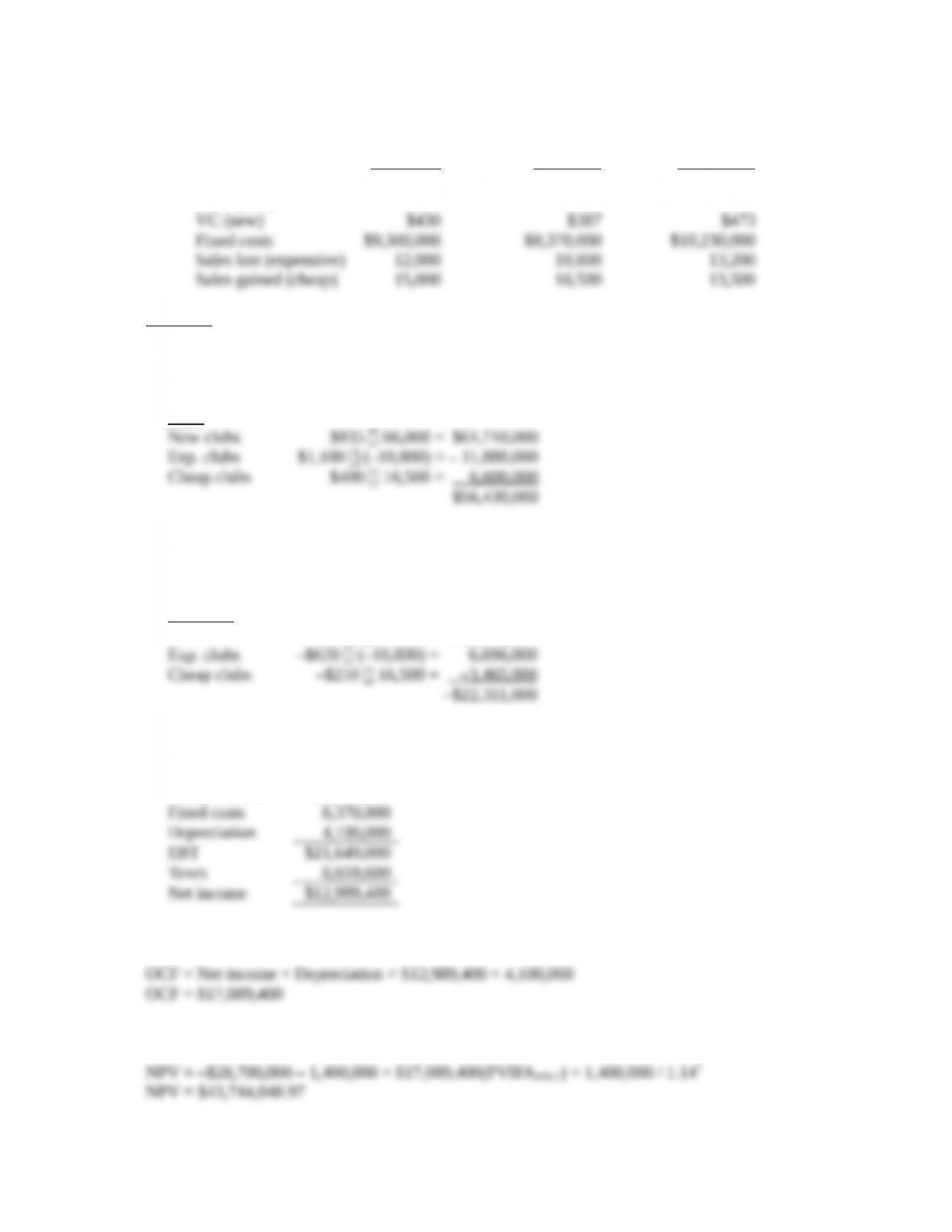
Base Case Best Case Worst Case
Unit sales (new) 60,000 66,000 54,000
Price (new) $850 $935 $765
Best-case
We will calculate the sales and variable costs first. Since we will lose sales of the expensive clubs
and gain sales of the cheap clubs, these must be accounted for as erosion. The total sales for the new
project will be:
Sales
For the variable costs, we must include the units gained or lost from the existing clubs. Note that the
variable costs of the expensive clubs are an inflow. If we are not producing the sets any more, we
will save these variable costs, which is an inflow. So:
Var. costs
New clubs –$387 66,000 = –$25,542,000
The pro forma income statement will be:
Sales $56,430,000
Variable costs 22,311,000
Using the bottom up OCF calculation, we get:
And the best-case NPV is:
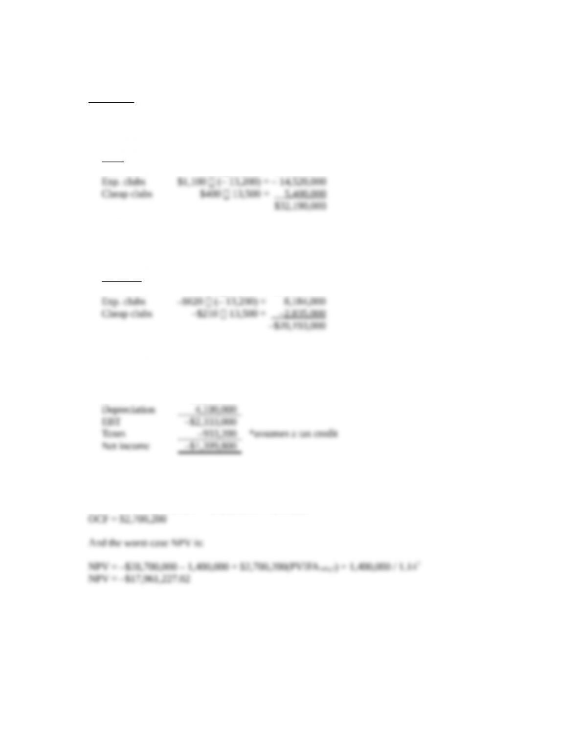
Worst-case
We will calculate the sales and variable costs first. Since we will lose sales of the expensive clubs
and gain sales of the cheap clubs, these must be accounted for as erosion. The total sales for the new
project will be:
Sales
New clubs $765 54,000 = $41,310,000
For the variable costs, we must include the units gained or lost from the existing clubs. Note that the
variable costs of the expensive clubs are an inflow. If we are not producing the sets any more, we
will save these variable costs, which is an inflow. So:
Var. costs
New clubs –$473 54,000 = –$25,542,000
The pro forma income statement will be:
Sales $32,190,000
Variable costs 20,193,000
Costs 10,230,000
Using the bottom up OCF calculation, we get:
OCF = NI + Depreciation = –$1,399,800 + 4,100,000
16. To calculate the sensitivity of the NPV to changes in the price of the new club, we need to change the
price of the new club. We will choose $860, but the choice is irrelevant as the sensitivity will be the
same no matter what price we choose.
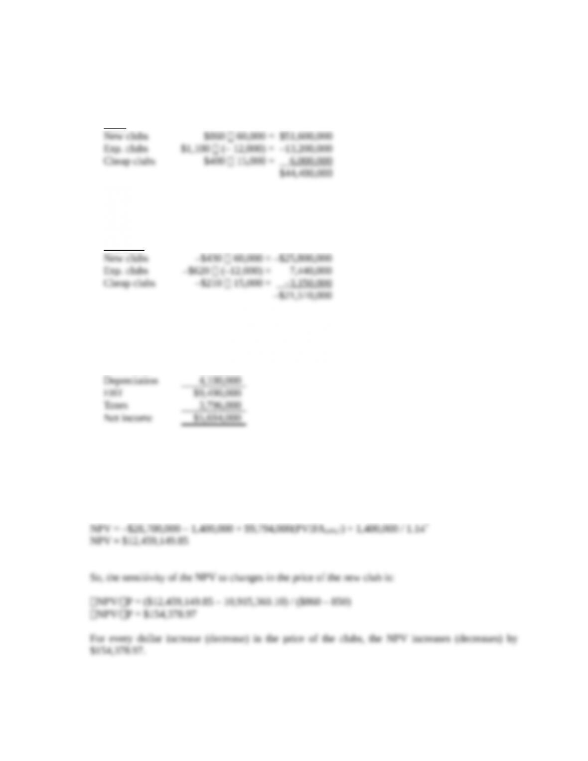
We will calculate the sales and variable costs first. Since we will lose sales of the expensive clubs
and gain sales of the cheap clubs, these must be accounted for as erosion. The total sales for the new
project will be:
Sales
For the variable costs, we must include the units gained or lost from the existing clubs. Note that the
variable costs of the expensive clubs are an inflow. If we are not producing the sets any more, we
will save these variable costs, which is an inflow. So:
Var. costs
The pro forma income statement will be:
Sales $44,400,000
Variable costs 21,510,000
Fixed costs 9,300,000
Using the bottom up OCF calculation, we get:
OCF = NI + Depreciation = $5,694,000 + 4,100,000
OCF = $9,794,000
And the NPV is:
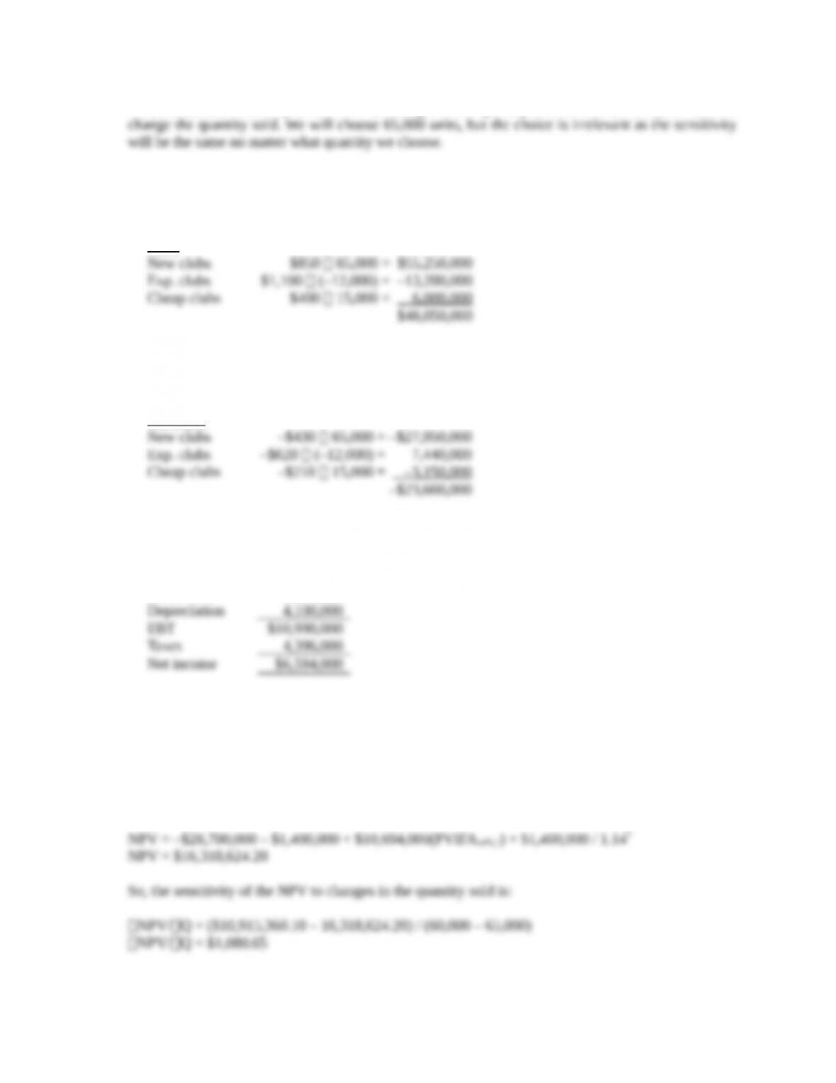
To calculate the sensitivity of the NPV to changes in the quantity sold of the new club, we need to
We will calculate the sales and variable costs first. Since we will lose sales of the expensive clubs
and gain sales of the cheap clubs, these must be accounted for as erosion. The total sales for the new
project will be:
Sales
For the variable costs, we must include the units gained or lost from the existing clubs. Note that the
variable costs of the expensive clubs are an inflow. If we are not producing the sets any more, we
will save these variable costs, which is an inflow. So:
Var. costs
The pro forma income statement will be:
Sales $48,050,000
Variable costs 23,660,000
Fixed costs 9,300,000
Using the bottom up OCF calculation, we get:
OCF = NI + Depreciation = $6,594,000 + 4,100,000
OCF = $10,694,000
The NPV at this quantity is:
17. a. The base-case NPV is:
b. We would abandon the project if the cash flow from selling the equipment is greater than the
present value of the future cash flows. We need to find the sale quantity where the two are
equal, so:
$820,000 = ($38)Q(PVIFA16%,9)
c. The $820,000 is the market value of the project. If you continue with the project in one year,
18. a. If the project is a success, the present value of the future cash flows will be:
PV future CFs = $38(9,500)(PVIFA16%,9)
PV future CFs = $1,662,962.34
From the previous question, if the quantity sold is 3,800, we would abandon the project, and the
cash flow would be $820,000. Since the project has an equal likelihood of success or failure in
b. If we couldn’t abandon the project, the present value of the future cash flows when the quantity
is 3,800 will be:
The gain from the option to abandon is the abandonment value minus the present value of the
cash flows if we cannot abandon the project, so:
Gain from option to abandon = $820,000 – 665,184.94
19. If the project is a success, the present value of the future cash flows will be:
If the sales are only 3,800 units, from Problem #17, we know we will abandon the project, with a
value of $820,000. Since the project has an equal likelihood of success or failure in one year, the
expected value of the project in one year is the average of the success and failure cash flows, plus the
cash flow in one year, so:
The NPV is the present value of the expected value in one year plus the cost of the equipment, so:
The gain from the option to expand is the present value of the cash flows from the additional units
sold, so:
We need to find the value of the option to expand times the likelihood of expansion. We also need to
find the value of the option to expand today, so:
20. a. The accounting breakeven is the aftertax sum of the fixed costs and depreciation charge divided
by the contribution margin (selling price minus variable cost). In this case, there are no fixed
costs, and the depreciation is the entire price of the press in the first year. So, the accounting
breakeven level of sales is:
b. When calculating the financial breakeven point, we express the initial investment as an
equivalent annual cost (EAC). The initial investment is the $20,000 in licensing fees. Dividing
the initial investment by the three-year annuity factor, discounted at 12 percent, the EAC of the
initial investment is:
Note, this calculation solves for the annuity payment with the initial investment as the present
value of the annuity, in other words:
Now we can calculate the financial breakeven point. Notice that there are no fixed costs or
depreciation. The financial breakeven point for this project is:
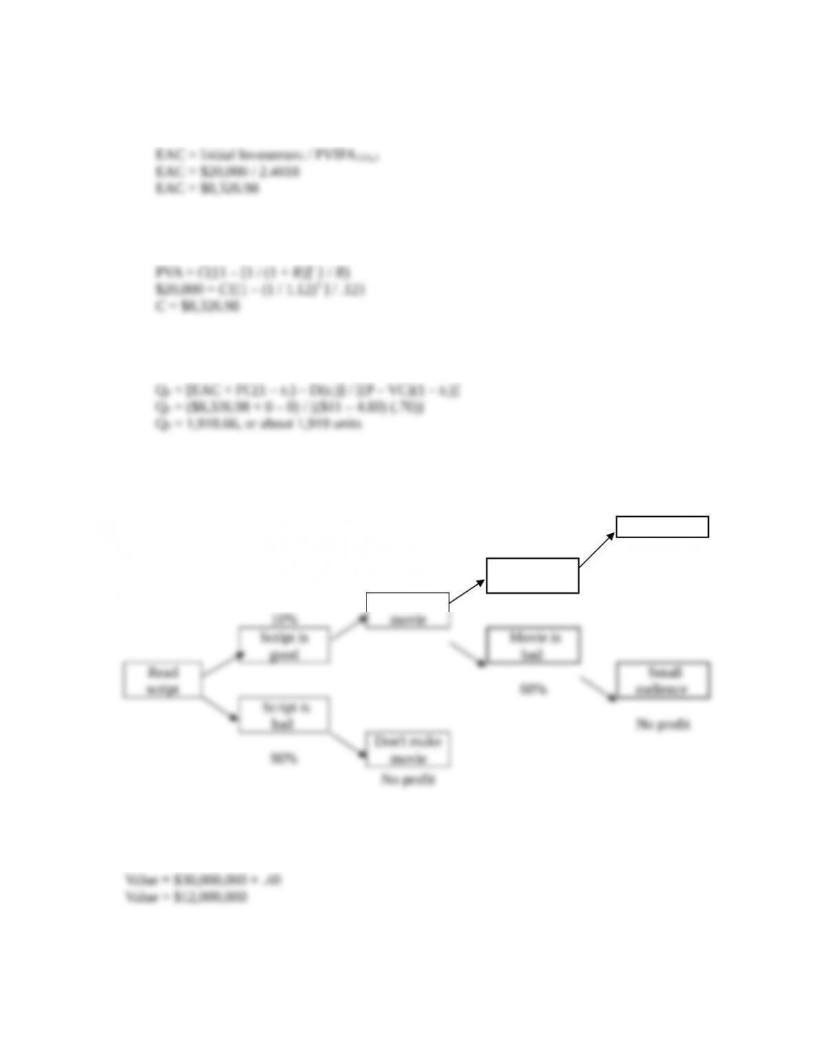
21. The payoff from taking the lump sum is $20,000, so we need to compare this to the expected payoff
from taking 1.5 percent of the profit. The decision tree for the movie project is:
Big audience
40% $30,000,000
Movie is
good
Make
The value of 1.5 percent of the profits is as follows. There is a 40 percent probability the movie is
good, and the audience is big, so the expected value of this outcome is:
The value if the movie is good, and has a big audience, assuming the script is good is:
This is the expected value for the studio, but the screenwriter will only receive 1.5 percent of this
amount, so the payment to the screenwriter will be:
22. We can calculate the value of the option to wait as the difference between the NPV of opening the
mine today and the NPV of waiting one year to open the mine. The remaining life of the mine is:
CF = 5,500($1,100) = $6,050,000
So, the NPV of opening the mine today is:
The PV of these cash flows is:
Price increase CF = $7,700,000(PVIFA12%,8) = $38,250,826.20
Price decrease CF = $4,950,000(PVIFA12%,8) = $24,589,816.85
So, the NPV is one year will be:
So, the value of the option to wait is: