
25. Certainty equivalent approach (LO13-1) Sheila Goodman recently received her MBA
from the Harvard Business School. She has joined the family business, Goodman Software
Products Inc., as vice president of finance.
She believes in adjusting projects for risk. Her father is somewhat skeptical but agrees
to go along with her. Her approach is somewhat different than the risk-adjusted discount
rate approach, but achieves the same objective.
She suggests that the inflows for each year of a project be adjusted downward for lack
of certainty and then be discounted back at a risk-free rate. The theory is that the
adjustment penalty makes the inflows the equivalent of risk-less inflows, and therefore a
risk-free rate is justified.
A table showing the possible coefficient of variation for an inflow and the associated
adjustment factor is shown next:
Coefficient
of Variation
Adjustment
Factor
0 – .25……….……. .90
.26 – .50……….……. .80
.51 – .75……….……. .70
.76 – 1.00……..……. .60
1.01 – 1.25…….……. .50
Assume a $184,000 project provides the following inflows with the associated coefficients
of variation for each year:
Year Inflow Coefficient of Variation
1
……………………….. $32,200 .12
2
……………………….. 59,500 .28
3
……………………….. 79,900 .45
4
……………………….. 59,200 .79
5
……………………….. 65,5600 1.15
a. Fill in the following table:
Year Inflow
Coefficient of
Variation
Adjustment
Factor
Adjusted
Inflow
1
……………..….…. $32,200 .12 ____________ ____________
2
……………..….…. 59,500 .28 ____________ ____________
3
……………..….…. 79,900 .45 ____________ ____________
4
……………..….…. 59,200 .79 ____________ ____________
5 65,600 1.15 ____________ ____________

……………..….….
b. If the risk-free rate is 5 percent, should this $184,000 project be accepted? Compute
the net present value of the adjusted inflows.
13-25. Solution:
Goodman Software Products
a. Adjusted Inflows
Year Inflow
Coefficient
of Variation
Adjustment
Factor
Adjusted
Inflow
1 $32,200 .12 .90 $28,980
2 59,500 .28 .80 47,600
b. Net Present Value
Year
Adjusted
Inflow
PVIF
at 5%
Present
Value
1 $28,980 .952 $ 27,589
2 47,600 .907 43,173
3 63,920 .864 55,227

COMPREHENSIVE PROBLEMS
Comprehensive Problem 1.
Gibson Appliance Co. (portfolio effect of a merger) (LO13-5) Gibson Appliance Co. is a very
stable billion-dollar company with a sales growth of about 7 percent per year in good or bad
economic conditions. Because of this stability (a coefficient of correlation with the economy
of +.4, and a standard deviation of sales of about 5 percent from the mean), Mr. Hoover, the vice
president of finance, thinks the company could absorb a small risky company that could add
quite a bit of return without increasing the company’s risk much. He is trying to decide which of
the two companies he will buy, using the following figures. Gibson’s cost of capital is
12 percent.
Genetic Technology Co.
(cost $80 million)
Silicon Microchip Co.
(cost $80 million)
Cash Flow
for 10 Years
($ millions) Probability
Cash Flow
for 10 Years
($ millions) Probability
$ 2 .2 $ 5 .2
8 .3 7 .2
16 .2 18 .3
25 .2 24 .3
40 .1
a. What is the expected cash flow from both companies?
b. Which company has the lower coefficient of variation?
c. Compute the net present value of each company.
d. Which company would you pick, based on the net present values?
e. Would you change your mind if you added the risk dimensions to the problem? Explain.
f. What if Genetic Technology Co. had a coefficient of correlation with the economy
of –.2, and Silicon Microchip Co. had one of +.5? Which of these companies would
give you the best portfolio effects for risk reduction?
g. What might be the effect of the acquisitions on the market value of Gibson Appliance
Co.’s stock?

CP 13-1 Solution:
Portfolio Effect of a Merger
Gibson Appliance Co.
a. Genetic Technology Co. Silicon Microchip Co.
D P DP D P DP
$ 2 .2 .4 $ 5 .2 1.0
8 .3 2.4 7 .2 1.4
Expected Value
of Cash Flows
$15.0
(million)
Expected Value
of Cash Flows
$15.0
(million)
b. Coefficient of variation for Genetic Technology Co.
D
D
( )D D–
2
( )D D–
P
2
( )D D–
P
$ 2 $15 $–13 $169 .2 $33.8
8 15 –7 49 .3 14.7
16 15 +1 1 .2 .2
25 15 +10 100 .2 20.0
CP 13-1. (Continued)
Coefficient of variation for Silicon Microchip Co.
D
D
( )D D–
2
( )D D–
P
2
( )D D–
P
$ 5 $15 $–103 $100 .2 $20.0
7 15 –8 64 .2 12.8
18 15 +3 9 .3 2.7
c. For both companies, the annual expected value is $15 million for
10 years. The cost is $80 million for either company.
Gibson has a cost of capital of 12 percent.
d. Based on present values, you could pick either company.
e. The only way one will win out over the other is if risk factors are
considered. Since Genetic Technology Co. has the higher coefficient
of variation, we would select the lower risk company––Silicon
f. Since Gibson Appliance Co. has a correlation coefficient with the
g. Because Gibson Appliance Co. is a stable billion-dollar company,
this investment of $80 million would probably not have a great
Comprehensive Problem 2.
Kennedy Trucking Company (investment decision based on probability analysis) (LO13-1)
Five years ago, Kennedy Trucking Company was considering the purchase of 60 new diesel
trucks that were 15 percent more fuel-efficient than the ones the firm is now using. Mr. Hoffman,
the president, had found that the company uses an average of 10 million gallons of diesel fuel per
year at a price of $1.25 per gallon. If he can cut fuel consumption by 15 percent, he will save
$1,875,000 per year (1,500,000 gallons times $1.25).
Mr. Hoffman assumed that the price of diesel fuel is an external market force that he cannot
control and that any increased costs of fuel will be passed on to the shipper through higher rates
endorsed by the Interstate Commerce Commission. If this is true, then fuel efficiency would save
more money as the price of diesel fuel rises (at $1.35 per gallon, he would save $2,025,000 in
total if he buys the new trucks). Mr. Hoffman has come up with two possible forecasts shown
next—each of which he feels has about a 50 percent chance of coming true. Under assumption
number 1, diesel prices will stay relatively low; under assumption number 2, diesel prices will
rise considerably. Sixty new trucks will cost Kennedy Trucking $5 million. Under a special
provision from the Interstate Commerce Commission, the allowable depreciation will be
25 percent in year 1, 38 percent in year 2, and 37 percent in year 3. The firm has a tax rate of
40 percent and a cost of capital of 10 percent.
a. First, compute the yearly expected price of diesel fuel for both assumption 1 (relatively
low prices) and assumption 2 (high prices) from the forecasts that follow.
Forecast for assumption 1 (low fuel prices):

Probability
(same for each year) Price of Diesel Fuel per Gallon
Year 1 Year 2 Year 3
.1 $ .80 $ .90 $1.00
.2 1.00 1.10 1.10
.3 1.10 1.20 1.30
.2 1.30 1.45 1.45
.2 1.40 1.55 1.60
Forecast for assumption 2 (high fuel prices):
Probability
(same for each year) Price of Diesel Fuel per Gallon
Year 1 Year 2 Year 3
.1 $1.20 $1.50 $1.70
.3 1.30 1.70 2.00
.4 1.80 2.30 2.50
.2 2.20 2.50 2.80
b. What will be the dollar savings in diesel expenses each year for assumption 1 and for
assumption 2?
c. Find the increased cash flow after taxes for both forecasts.
d. Compute the net present value of the truck purchases for each fuel forecast
assumption and the combined net present value (that is, weigh the NPV by .5).
e. If you were Mr. Hoffman, would you go ahead with this capital investment?
f. How sensitive to fuel prices is this capital investment?
CP 13-2 Solution:
Investment Decision Based on Probability Analysis
Kennedy Trucking Company
a. Assumption One:
Yr.1 Yr.2 Yr.3
Probability D DP D DP D DP
.1 $0.80 .08 $0.9
0
.09 $1.00 .10
.2 1.00 .20 1.10 .22 1.10 .22
Assumption Two:
Yr.1 Yr.2 Yr.3
Probability D DP D DP D DP
.1 $1.2
0
.12 $1.5
0
.15 $1.7
0
.17
.3 1.30 .39 1.70 .51 2.00 .60
n
n
13-CP 2. (Continued)
b. Assumption One:
Yr.
Expected
Cost/Gal.
# of Gals.
Without
Efficiency = Cost
% Savings
with
Efficiency
Total
$ Saved
1 $1.15 10 million $11,500,000 15% $1,725,000
Assumption Two:
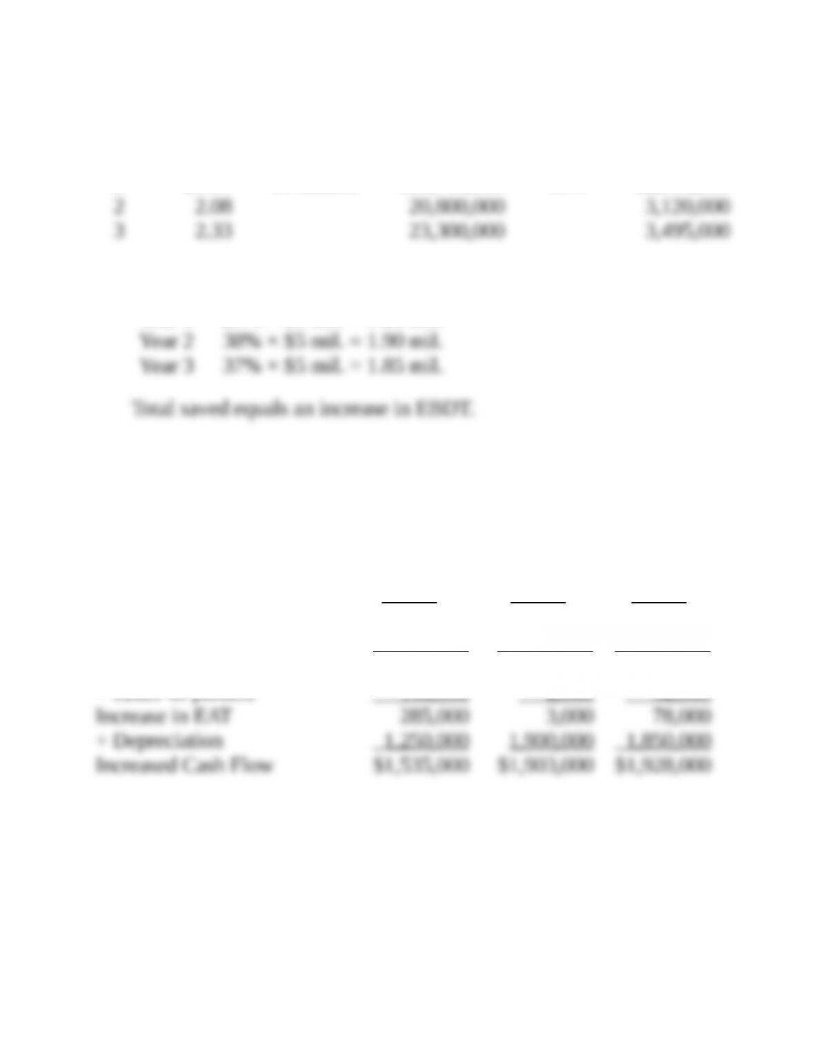
Yr.
Expected
Cost/Gal.
# of Gals.
without
Efficiency = Cost
% Savings
with
Efficiency
Total
$ Saved
1 $1.67 10 million $16,700,000 15% $2,505,000
c. First, compute annual depreciation. Then, proceed to the analysis.
Year 1 25% × $5 mil. = 1.25 mil.
13-CP 2. (Continued)
Assumption One:
Year 1 Year 2 Year 3
Increase in EBDT $1,725,000 $1,905,000 $1,980,000
– Depreciation 1,250,000 1,900,000 1,850,000
Increase in EBT 475,000 5,000 130,000
– Taxes 40 percent 190,000 2,000 52,000
Assumption Two:
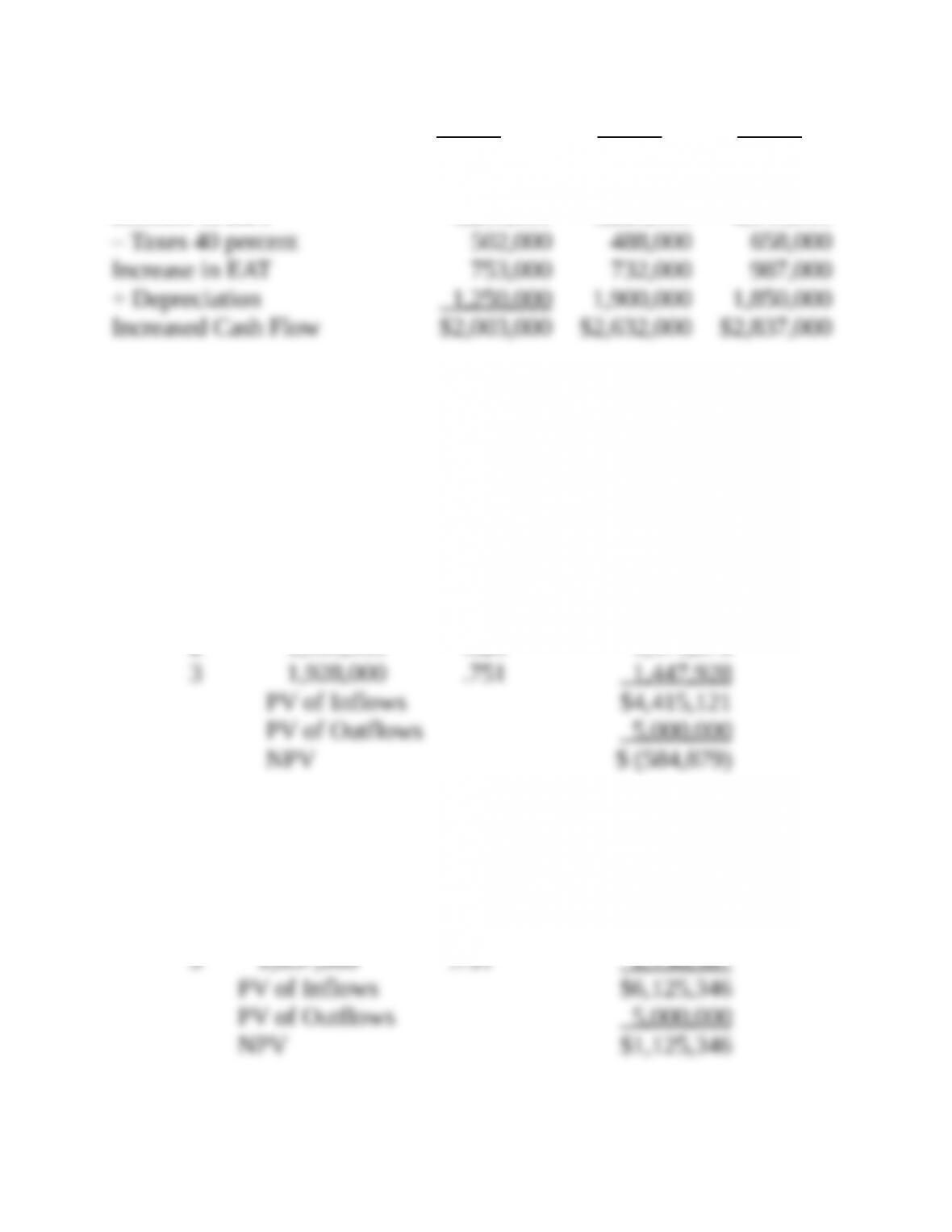
Year 1 Year 2 Year 3
Increase in EBDT $2,505,000 $3,120,000 $3,495,000
– Depreciation 1,250,000 1,900,000 1,850,000
Increase in EBT 1,255,000 1,220,000 1,645,000
13-CP 2. (Continued)
d. Present Value
Assumption One:
Year Cash Flow PVIF @ 10% Present Value
1 $1,535,000 .909 $1,395,315
2 1,903,000 .826 1,571,878
Assumption Two:
Year Cash Flow PVIF @ 10% Present Value
1 $2,003,000 .909 $1,820,727
2 2,632,000 .826 2,174,032
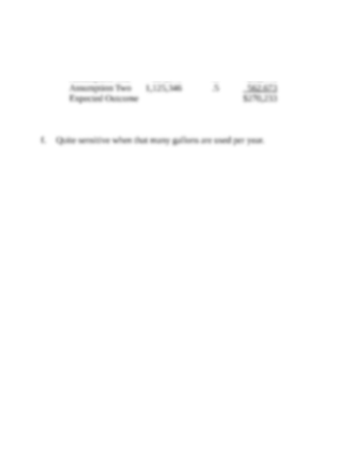
Combined NPV:
Outcome NPV Probability
Assumption One –584,879 .5 –292,440
e. Yes—The combined expected value of the outcomes is positive.