
Chapter 13: Risk and Capital Budgeting
13-15. Solution:
Discount Rate
Years 5% 20%
1 .952 .833
The impact of a high discount rate is much greater on long-term
value. For example, after the first year, the high rate discount
16. Expected value with net present value (LO13-1) Debby’s Dance Studios is considering
the purchase of new sound equipment that will enhance the popularity of its aerobics
dancing. The equipment will cost $27,900. Debby is not sure how many members the new
equipment will attract, but she estimates that her increased annual cash flows for each of
the next five years will have the following probability distribution. Debby’s cost of capital
is 15 percent.
Cash Flow Probability
$4,570
…………………………….….…… .1
5,550
…………………………….….…… .3
7,400
…………………………….….…… .4
9,930
…………………………….….…… .2
a. What is the expected value of the cash flow? The value you compute will apply to
each of the five years.
b. What is the expected net present value?
c. Should Debby buy the new equipment?
Chapter 13: Risk and Capital Budgeting
13-16. Solution:
Debby’s Dance Studios
a. Expected Cash Flow
Cash Flow P
$4,570 × .1 $ 457
5,550 × .3 1,665
b. Net Present Value (Appendix D)
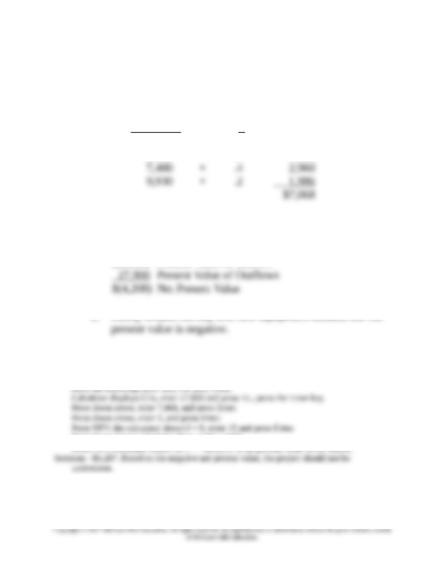
$7,068 × 3.352 (PVIFA @ 15%, n = 5) =
$23,692 Present Value of Inflows
c. Debby should not buy this new equipment because the net
Calculator solution:
b.
Find the PV of cash inflow using a financial calculator at 15 percent:
Press down arrow; calculator shows NPV = 0.00.
17. Deferred cash flows and risk-adjusted discount rate Highland Mining and Minerals Co.
is considering the purchase of two gold mines. Only one investment will be made. The
Australian gold mine will cost $1,649,000 and will produce $353,000 per year in years 5
Chapter 13: Risk and Capital Budgeting
through 15 and $503,000 per year in years 16 through 25. The U.S. gold mine will cost
$2,054,000 and will produce $282,000 per year for the next 25 years. The cost of capital is
13 percent.
a. Which investment should be made? (Note: In looking up present value factors for this
problem, you need to work with the concept of a deferred annuity for the Australian
mine. The returns in years 5 through 15 actually represent 11 years; the returns in
years 16 through 25 represent 10 years.)
b. If the Australian mine justifies an extra 2 percent premium over the normal cost of
capital because of its riskiness and relative uncertainty of cash flows, does the
investment decision change?
13-17. Solution:
Highland Mining and Minerals Co.
a. Calculate the net present value for each project.
The Australian Mine
Years
Cash
Flow n Factor PVIFA@13%
Present
Value
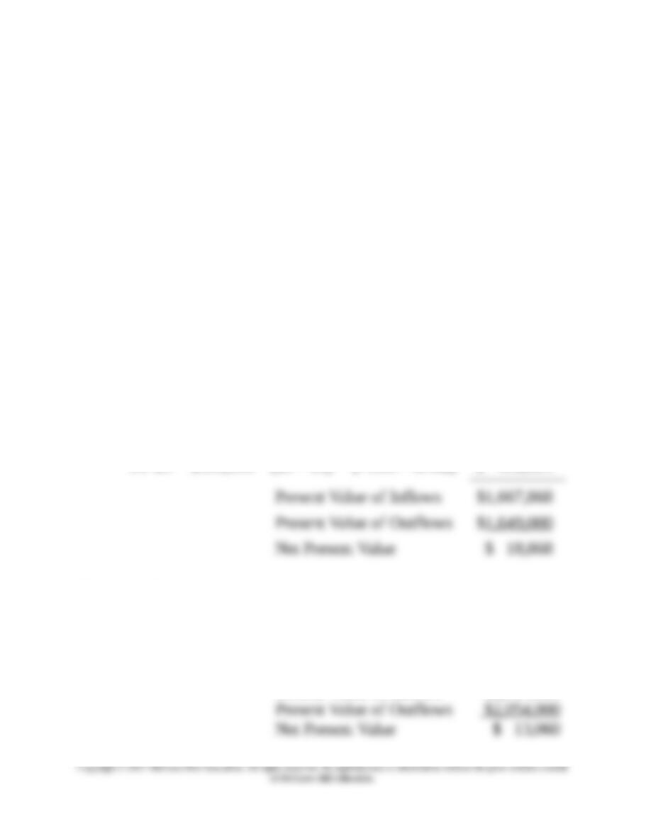
5–15 $353,000 (15 – 4) (6.462 – 2.974) $1,231,264
16–25 $503,000 (25 – 15) (7.330 – 6.462) $ 436,604
The U.S. Mine
Years Cash Flow n Factor PVIFA@13%
Present
Value
1–25 $282,000 (25) 7.330 $2,067,060
Present Value of Inflows $2,067,060
Chapter 13: Risk and Capital Budgeting
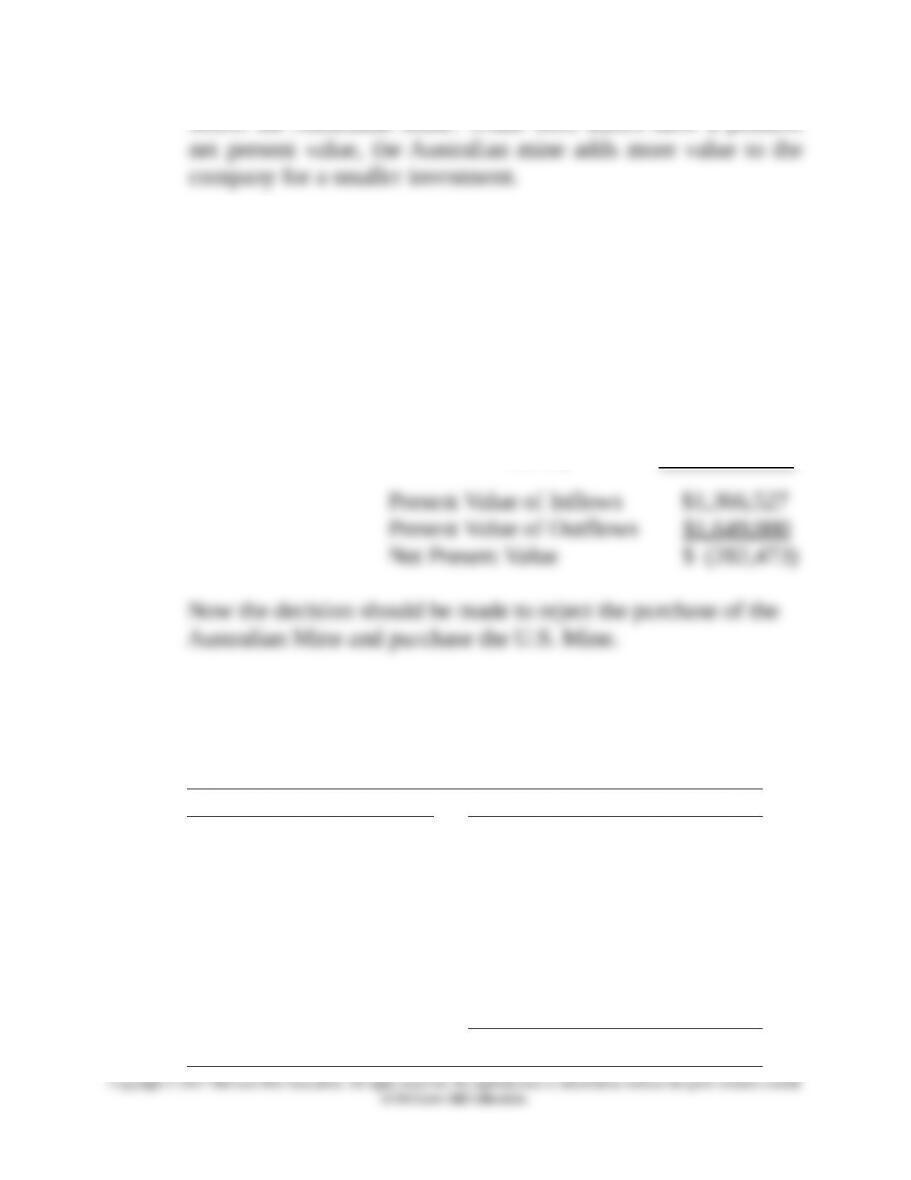
Select the Australian Mine. While both mines have a positive
b. Recalculate the net present value of the Australian Mine at a
15 percent discount rate.
Years Cash Flow n Factor PVIFA @ 15%
Present
Value
5–15 $353,000 (15 – 4) (5.847 –
2.855)
$ 1,056,176
16–25 $503,000 (25 – 15) (6.464 –
5.847)
$ 310,351
18. Coefficient of variation and investment decision (LO13-1) Mr. Sam Golff desires to
invest a portion of his assets in rental property. He has narrowed his choices down to two
apartment complexes, Palmer Heights and Crenshaw Village. After conferring with the present
owners, Mr. Golff has developed the following estimates of the cash flows for these properties:
Palmer Heights Crenshaw Village
Yearly Aftertax
Cash Inflow
(in thousands) Probability
Yearly Aftertax Cash
Inflow (in
thousands) Probability
$70
……………………………. .2 $75………….... .2
75
……………………………. .2 80………….... .3
90
……………………………. .2 90………….... .4
105
……………………………. .2 100………….. .1
110
……………………………. .2
Chapter 13: Risk and Capital Budgeting
a. Find the expected cash flow from each apartment complex.
b. What is the coefficient of variation for each apartment complex?
c. Which apartment complex has more risk?
13-18. Solution:
Mr. Sam Golff
D DP=
å
Palmer Heights Crenshaw Village
D P DP D P DP
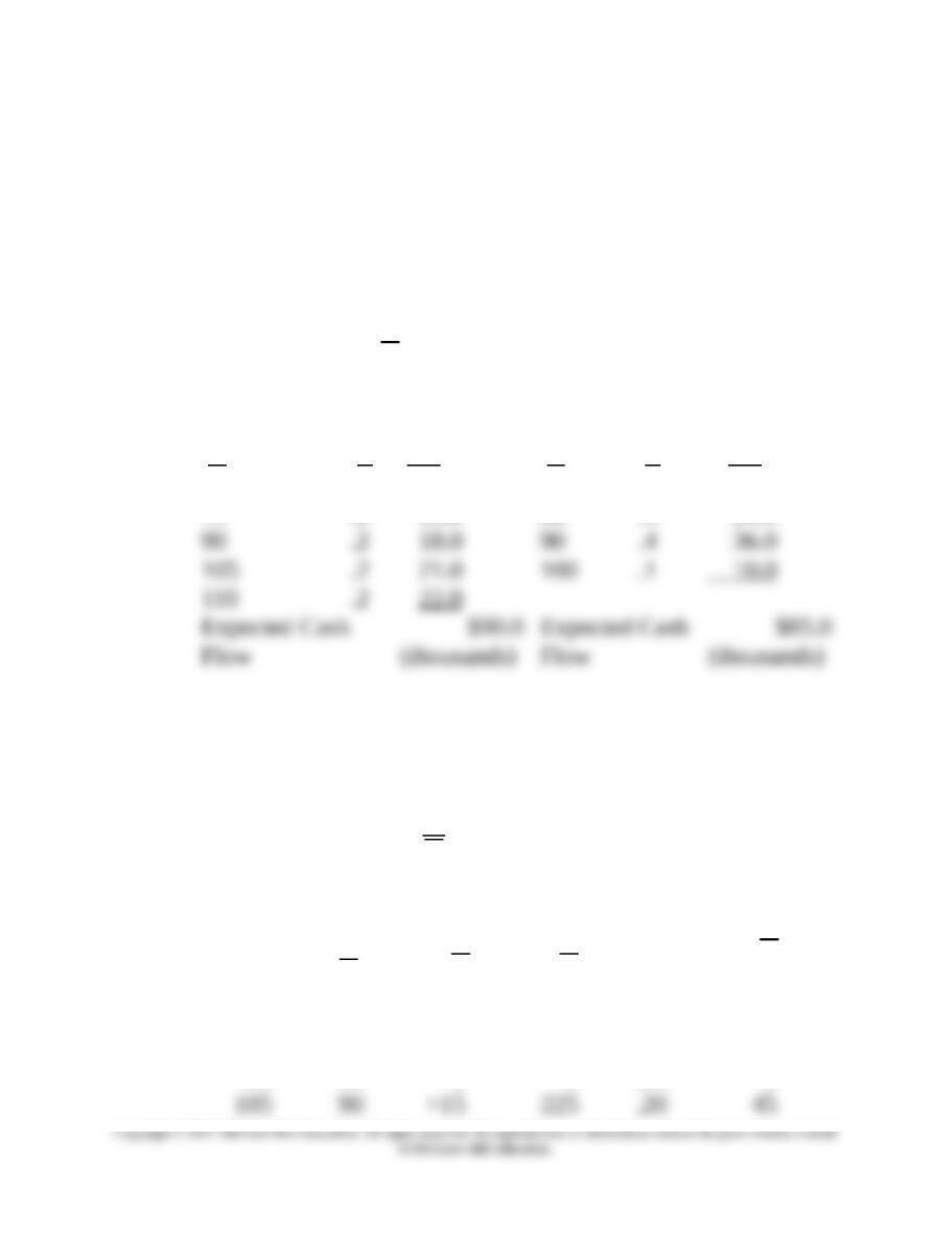
70 .2 $14.0 75 .2 $ 15.0
75 .2 15.0 80 .3 24.0
a. First find the standard deviation and then the coefficient of
variation.
V
D
s
=
Palmer Heights
D
D
( )D D–
2
( )D D–
P
2
( )D D–
P
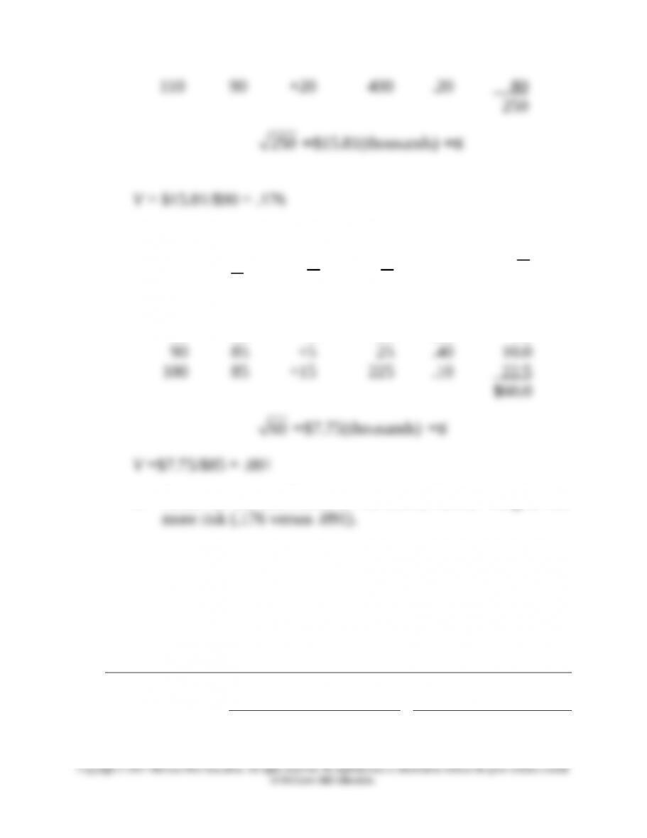
$70 $90 $–20 $400 .20 80
75 90 –15 225 .20 45
90 90 0 0 .20 0
Chapter 13: Risk and Capital Budgeting
Crenshaw Village
D
D
( )D D–
2
( )D D–
P
2
( )D D–
P
$75 $85 $–10 $100 .20 20.0
80 85 –5 25 .30 7.5
b. Based on the coefficient of variation, Palmer Heights has
19. Decision-tree analysis (LO13-4) Allison’s Dresswear Manufacturers is preparing a
strategy for the fall season. One alternative is to expand its traditional ensemble of wool
sweaters. A second option would be to enter the cashmere sweater market with a new line
of high-quality designer label products. The marketing department has determined that the
wool and cashmere sweater lines offer the following probability of outcomes and related
cash flows:
Expand Wool
Sweaters Line
Enter Cashmere
Sweaters Line
Expected
Sales
Probability
Present Value
of Cash Flows
from Sales Probability
Present
Value of
Cash Flows

Chapter 13: Risk and Capital Budgeting
from Sales
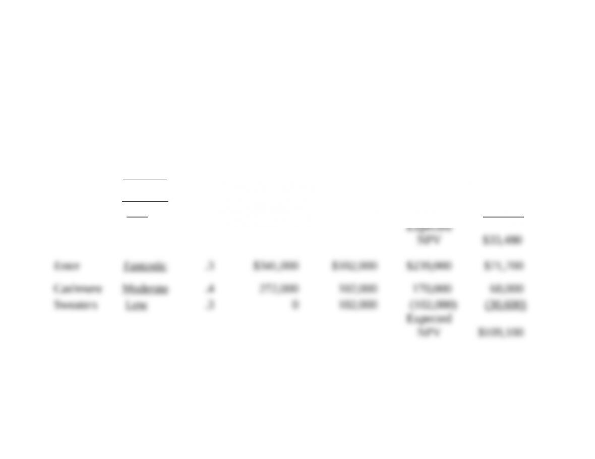
Fantastic….…….......... .5 $221,000 .3 $341,000
Moderate……………….. .2 192,000 .4 272,000
Low………………………. .3 88,600 .3 0
The initial cost to expand the wool sweater line is $142,000. To enter the cashmere sweater
line, the initial cost in designs, inventory, and equipment is $102,000.
a. Diagram a complete decision tree of possible outcomes similar to Figure 13-8. Note
that you are dealing with thousands of dollars rather than millions. Take the analysis
all the way through the process of computing expected NPV (the last column for each
investment).
b. Given the analysis in part a, would you automatically make the investment indicated?
Chapter 13: Risk and Capital Budgeting
13-19. Solution:
Allison’s Dresswear Manufacturers
a. (1) (2) (3) (4) (5) (6)
Expected
Sales Probability
Present Value
of Cash Flows
from Sales Initial Cost
NPV
(3) – (4)
Expected
NPV
(2) × (5)
Expand Fantastic .5 $221,000 $142,000 $79,000 $39,500
Wool Moderate .2 192,000 142,000 50,000 10,000
Sweaters Low .3 88,600 142,000 (53,400) (16,020)
13-8

Chapter 13: Risk and Capital Budgeting
b. The indicated investment, based on the expected NPV, is in the Cashmere sweater line.
13-9

Chapter 13: Risk and Capital Budgeting
20. Probability analysis with a normal curve distribution (LO13-4) When returns from a
project can be assumed to be normally distributed, such as those shown in Figure 13-6
(represented by a symmetrical, bell-shaped curve), the areas under the curve can be
determined from statistical tables based on standard deviations. For example, 68.26 percent
of the distribution will fall within one standard deviation of the expected value (
D
± 1σ).
Similarly, 95.44 percent will fall within two standard deviations (
D
± 2σ), and so on. An
abbreviated table of areas under the normal curve is shown next.
Number of σ’s
from Expected Value + or – + and –
0.5
……………………….….…… 0.1915 0.3830
1.0
……………………….….…… 0.3413 0.6826
1.5
……………………….….…… 0.4332 0.8664
1.65
……………………….….…… 0.4505 0.9010
2.0
……………………….….…… 0.4772 0.9544
Assume Project A has an expected value of $24,000 and a standard deviation (σ) of $4,800.
a. What is the probability that the outcome will be between $16,800 and $31,200?
b. What is the probability that the outcome will be between $14,400 and $33,600?
c. What is the probability that the outcome will be at least $14,400?
d. What is the probability that the outcome will be less than $31,900?
e. What is the probability that the outcome will be less than $19,200 or greater than
$26,400?
13-20. Solution:
a. Expected Value = $24,000, σ = $4,800
$16,800 > $24,000 < $31,200
Chapter 13: Risk and Capital Budgeting
13-11
Chapter 13: Risk and Capital Budgeting
13-20. (Continued)
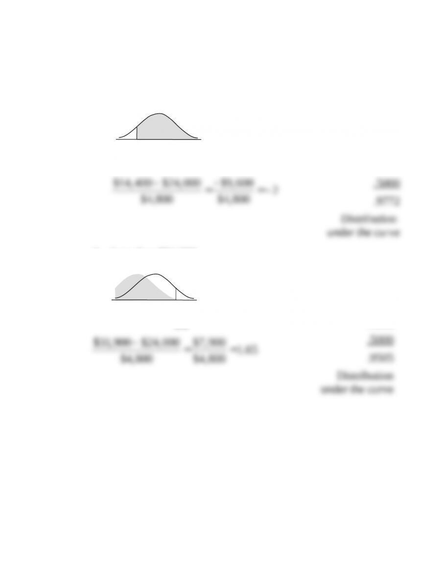
c. At least $14,400
d. Less than $31,900
13-12
$14,4
00
$31,9
00
.4772
.4505