Gale Force Surfing Case 5
Working Capital—Level vs. Seasonal Production
Purpose: The case forces the student to view the impact of level versus seasonal production on inventory
levels, bank loan requirements, and profitability. It also considers the efficiencies (or inefficiencies)
covered by the different production plans. The computations in the case are parallel to Table 6-1 through
Table 6-5 in the text, with the only difference being that seasonal production rather than level production
is being utilized. The case allows the student to properly track the movement of cash flow through the
production process.
Relation to Text: The case should follow Chapter 6.
Complexity: The case involves numerous computations and may require 2 hours.
Solutions
1. New Tables 1 through 5, with Tim’s suggestion implemented, are shown in the following pages.
Observe that the inventory level is now constant at 400 units or $800,000 a month because all units
2. New Table 5 shows the new cumulative loan balances and the interest expenses incurred each month.
3. The first step is to compute total sales. Using the second row of Table 3 (either the old or new table),
GALE FORCE SURFING (With Tim’s suggestion implemented)
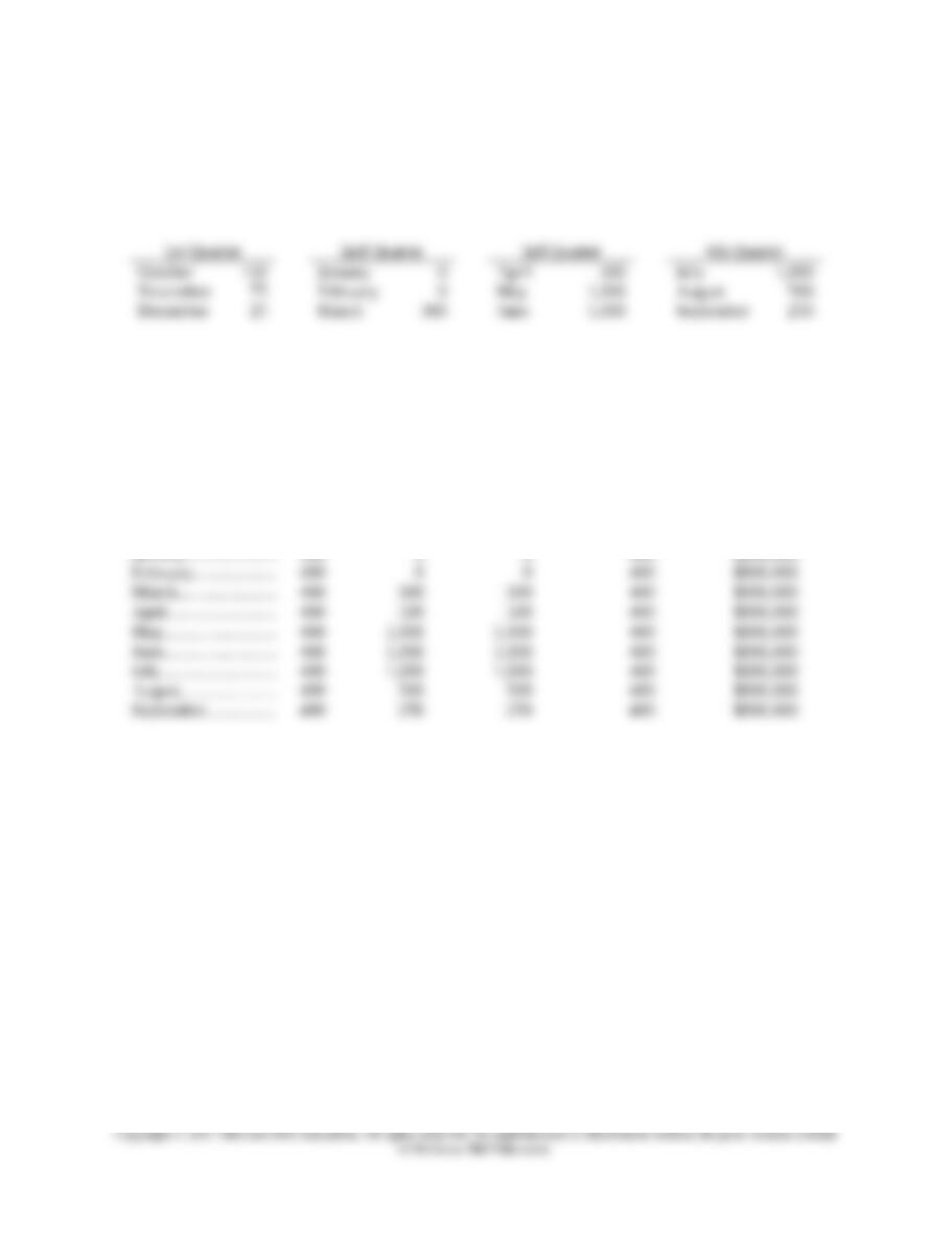
TABLE 1. SALES FORECAST (in units)
TABLE 2. PRODUCTION SCHEDULE AND INVENTORY (seasonal production)
Beginning
Inventory
Production
this Month Sales
Ending
Inventory
Inventory
($2,000 per
unit)
October…..…..…....... 400 + 50 – 150 = 400 $800,000
November…............. 400 75 75 400 $800,000
December…….…….... 400 25 25 400 $800,000
January……..……...…. 400 0 0 400 $800,000
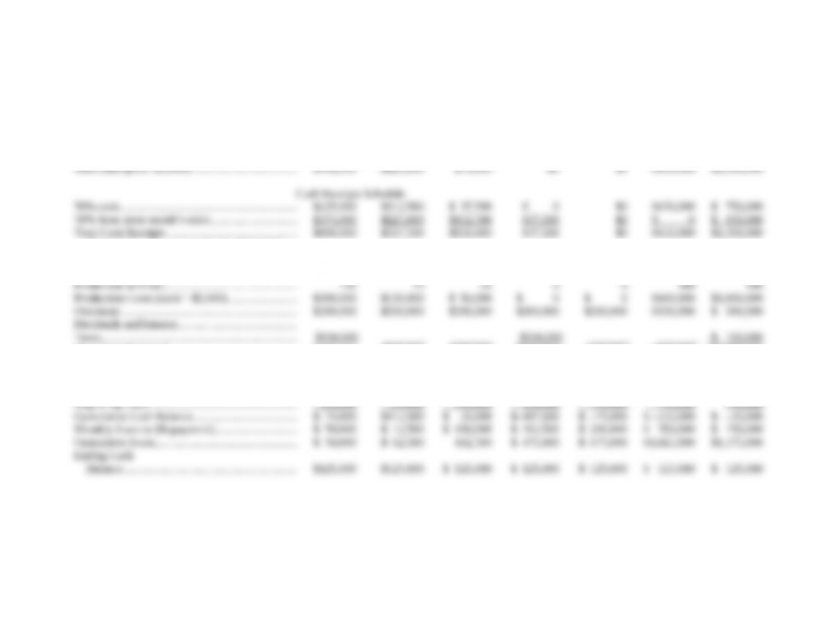
TABLE 3. SALES FORECAST, CASH RECEIPTS AND PAYMENTS, AND CASH BUDGET
October November December January February March April
Sales Forecast
Sales (units)…….……..……..…….……..……..…....…. 150 75 25 0 0 300 500
(Note: Sept. sales assumed to be $750,000)
Cash Payments Schedule
Total Cash Payments………….……..……..……..……. $650,000 $350,000 $250,000 $350,000 $200,000 $800,000 $1,350,000
Cash Budget—Required Minimum Balance is $125,000
Cash Flow…….……..……..…….……..……..……...….. $–50,000 $–12,500 $–100,000 $–312,500 $–200,000 $ –350,000 $ –150,000
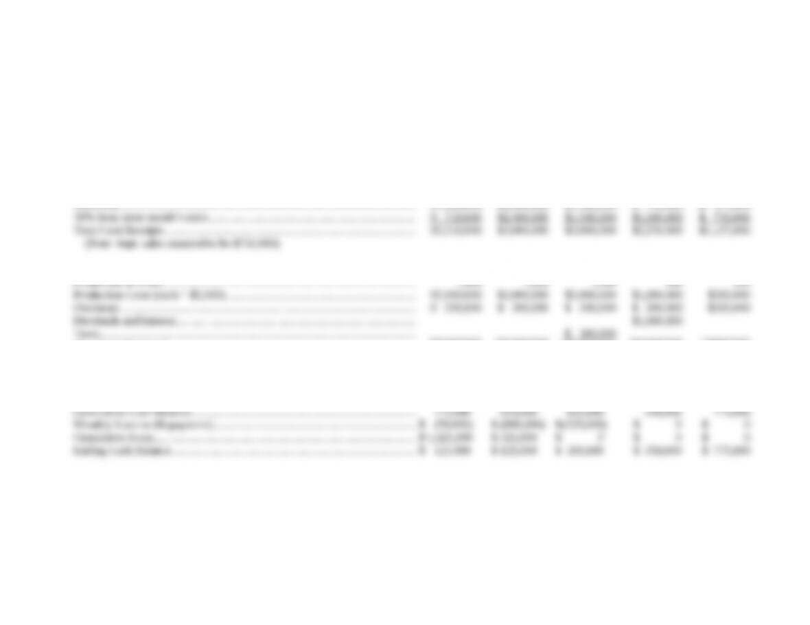
TABLE 3. (Continued) SALES FORECAST, CASH RECEIPTS AND PAYMENTS, AND CASH BUDGET
May June July August September
Sales Forecast
Sales (units)………………………………………………………………………………………. 1,000 1,000 1,000 500 250
Sales (unit price: $3,000)….……..……..……..…….……..……..…....…....…..…...... $3,000,000 $3,000,000 $3,000,000 $1,500,000 $750,000
Cash Receipts Schedule
Cash Payments Schedule
Total Cash Payments…………………………………………………………………..……... $2,200,000 $2,200,000 $2,500,000 $2,200,000 $700,000
Cash Budget—Required Minimum Balance is $125,000
Cash Flow…………………………………………………………………………..….…….….. $ 50,000 $ 800,000 $ 500,000 $ 50,000 $ 425,000
Beginning Cash…………………………………………………………………………..….…. 125,000 125,000 125,000 300,000 350,000
TABLE 4. TOTAL CURRENT ASSETS, FIRST YEAR
Total
January……..……...…. $125,000 $ 0 $800,000 $ 925,000
February……..…....…. $125,000 $ 0 $800,000 $ 925,000
March……..……..……. $125,000 $ 450,000 $800,000 $1,375,000
April…………..……..... $125,000 $ 750,000 $800,000 $1,675,000
May…….……..…....…. $125,000 $1,500,000 $800,000 $2,425,000
TABLE 5. CUMULATIVE LOAN BALANCE AND INTEREST EXPENSE
(17% per month)
October Novembe
r
Decembe
r
January February March April
Expense at
12.00%…..…..... $ 500 $ 625 $ 1,625 $ 4,750 $ 6,750 $ 10,250 $ 11,750
(Prime, 8.0%,