4. Suppose the following data describe the demand for liquid diet beverages:
Price $11 $10 $9 $8 $7 $6 $5 $4 $3 $2
Quantity 7 10 13 16 19 22 25 28 31 34
Demanded
Five identical, perfectly competitive firms are producing these beverages. The cost
of producing these beverages at each firm is the following:
Quantity 0 1 2 3 4 5 6 7 8 9 10
TC $5 $8 $10 $13 $17 $22 $28 $36 $45 $55 $67
(a) What price will prevail in this market?
(b) What quantity is produced?
(c) How much profit (loss) does each firm make?
(d) What happens to price if two more identical firms enter the market?
(LO 09-01)
Answers:
Feedback:
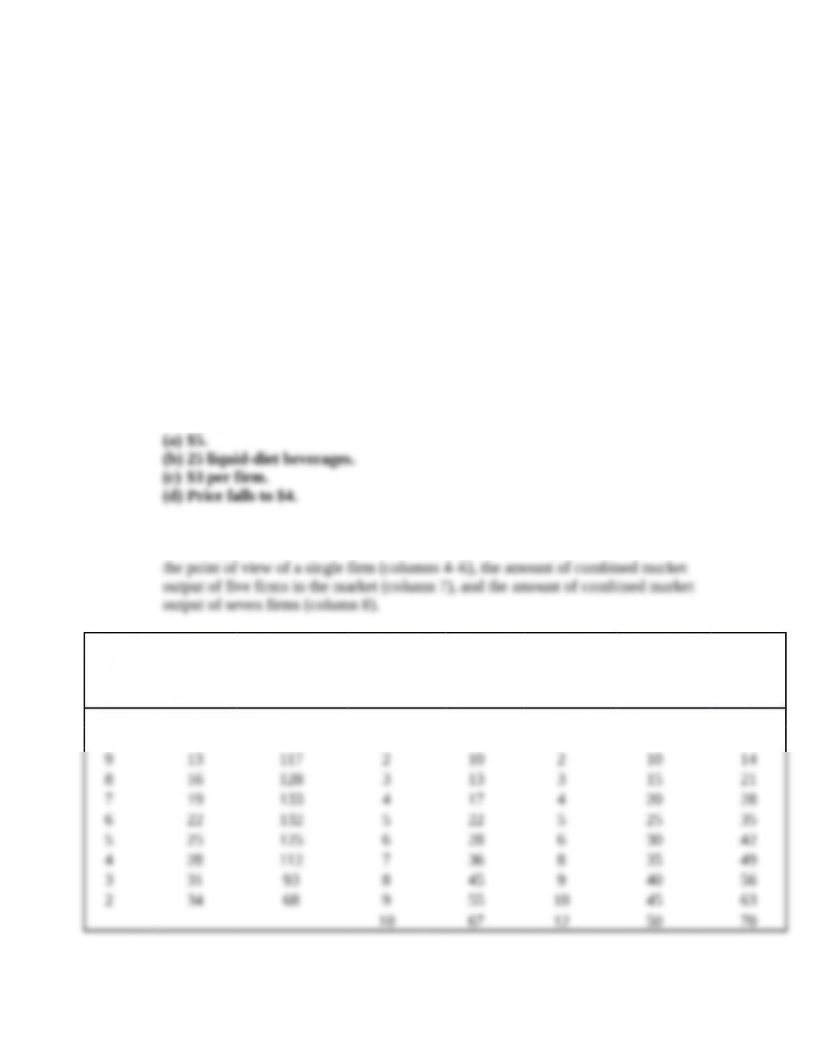
Following are the demand data for the market (columns 1–3), the cost data from
Price
Quantity
Demande
d
Total
Revenue
Quantity
Produce
d (One
Firm)
Total
Cost Marginal
Cost
Quantity
Produced
(Five
Firms)
Quantity
Produced
(Seven
Firms)
11 7 77 0 5 – – –
10 10 100 1 8 3 5 7
1
© 2016 by McGraw-Hill Education. This is proprietary material solely for authorized instructor use. Not authorized for sale or
distribution in any manner. This document may not be copied, scanned, duplicated, forwarded, distributed, or posted on a website, in
whole or part.
(a) The equilibrium that will prevail in the market is the price at which quantity
(b) At an equilibrium price of $5, the quantity demanded is 25 units, and since the
(c) Total Profit = Total Revenue – Total Cost. At equilibrium output (25 units),
(d) Again, the equilibrium that will prevail in the market is the price at which
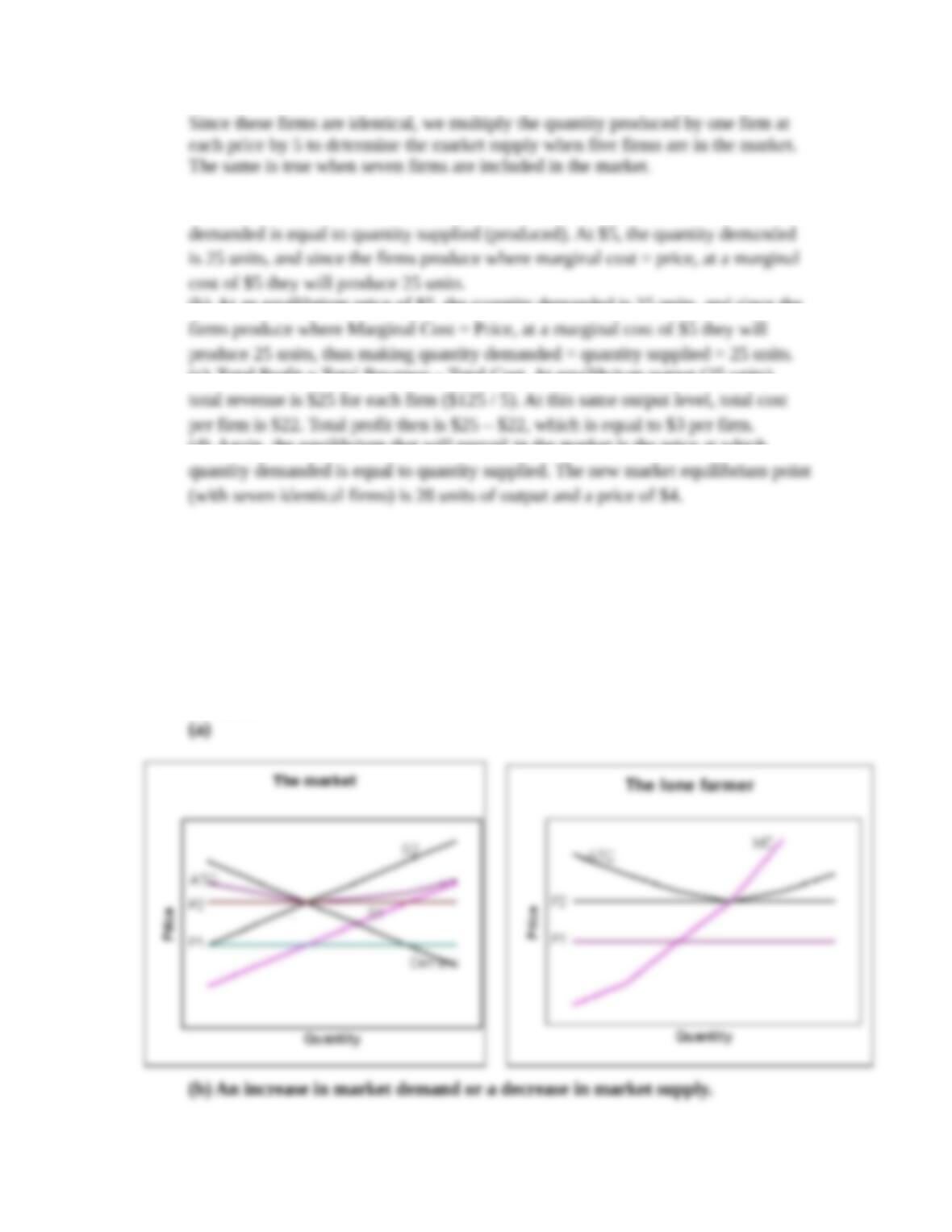
5. Suppose the typical catfish farmer was incurring an economic loss at the prevailing
price p1.
(a) Illustrate these losses on the firm and market graphs.
(b) What forces would raise the price?
(c) What price would prevail in long-term equilibrium? Illustrate your answers on
the graphs. (LO 09-03)
Answers:
2
© 2016 by McGraw-Hill Education. This is proprietary material solely for authorized instructor use. Not authorized for sale or
distribution in any manner. This document may not be copied, scanned, duplicated, forwarded, distributed, or posted on a website, in
whole or part.
(c) P2 shown above.
Feedback:
(a) The firm incurs a loss when its average total cost is more than the total revenue
(b) Any force that decreases supply or increases demand would raise the market
(c) The decrease in catfish supply would raise price levels to a new equilibrium
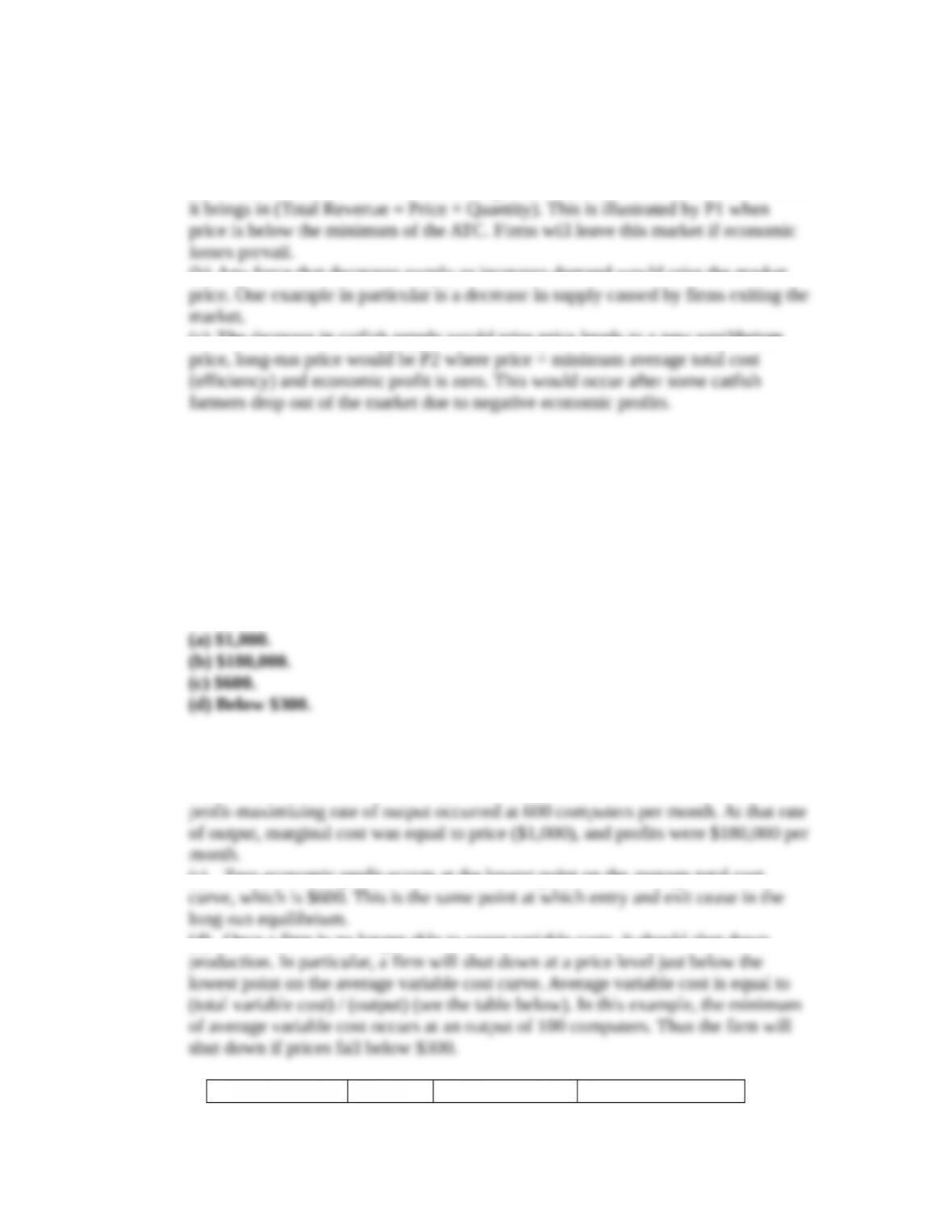
6. According to Table 9.1,
(a) What was the prevailing computer price in 1978?
(b) How much total profit did the typical firm earn?
(c) At what price would profits have been zero?
(d) At what price would the firm have shut down?
(LO 09-03)
Answers:
Feedback:
(a) According to Table 9.1, the prevailing computer price in 1978 was $1,000.
(b) Producers seek the rate of output at which total profit is maximized. The
(c) Zero economic profit occurs at the lowest point on the average total cost
(d) Once a firm is no longer able to cover variable costs, it should shut down
Output per Total Total Variable Average Variable
3
© 2016 by McGraw-Hill Education. This is proprietary material solely for authorized instructor use. Not authorized for sale or
distribution in any manner. This document may not be copied, scanned, duplicated, forwarded, distributed, or posted on a website, in
whole or part.

Month Cost Cost Cost
0 $60,000 $0 —
100 $90,000 $30,000 $300
$130,00
7. According to the World View on page 193,
(a) How many brands entered the flat-panel TV market between 2002 and 2007?
(b) What will economic profit be in the long run?
(c) Will the number of firms producing TVs (A) increase, (B) decrease, or (C) stay
the same between now and then?
(LO 09-02)
Answers:
Feedback:
(a) According to the World View, 102 LCD television brands were available in
(b) If the short-run equilibrium is profitable (price > minimum average total cost),
(c) More firms will enter this market in the long run. Low barriers to entry—parts
4
© 2016 by McGraw-Hill Education. This is proprietary material solely for authorized instructor use. Not authorized for sale or
distribution in any manner. This document may not be copied, scanned, duplicated, forwarded, distributed, or posted on a website, in
whole or part.
8. Suppose that the monthly market demand schedule for Frisbees is
Price $8 $7 $6 $5 $4 $3 $2 $1
Quantity
Demanded 1,000 2,000 4,000 8,000 16,000 32,000 64,000 128,000
Suppose further that the marginal and average costs of Frisbee production for
every competitive firm are
Rate of Output 100 200 300 400 500 600
Marginal Cost $2.00 $3.00 $4.00 $5.00 $6.00 $7.00
Average Total Cost $2.00 $2.50 $3.00 $3.50 $4.00 $4.50
Finally, assume that the equilibrium market price is $6 per Frisbee.
(a) Draw the cost curves of the typical firm and identify its profit-maximizing rate
of output and its total profits.
(b) Draw the market demand curve and identify market equilibrium.
(c) How many Frisbees are being sold?
(d) How many (identical) firms are initially producing Frisbees?
(e) How much profit is the typical firm making?
(f) In view of the profits being made, more firms will enter into Frisbee
production, shift the market supply curve to the right, and push price down. At
what equilibrium price are all profits eliminated?
(g) How many firms will be producing Frisbees at this long-term price?
(LO 09-04)
Answers:
5
© 2016 by McGraw-Hill Education. This is proprietary material solely for authorized instructor use. Not authorized for sale or
distribution in any manner. This document may not be copied, scanned, duplicated, forwarded, distributed, or posted on a website, in
whole or part.
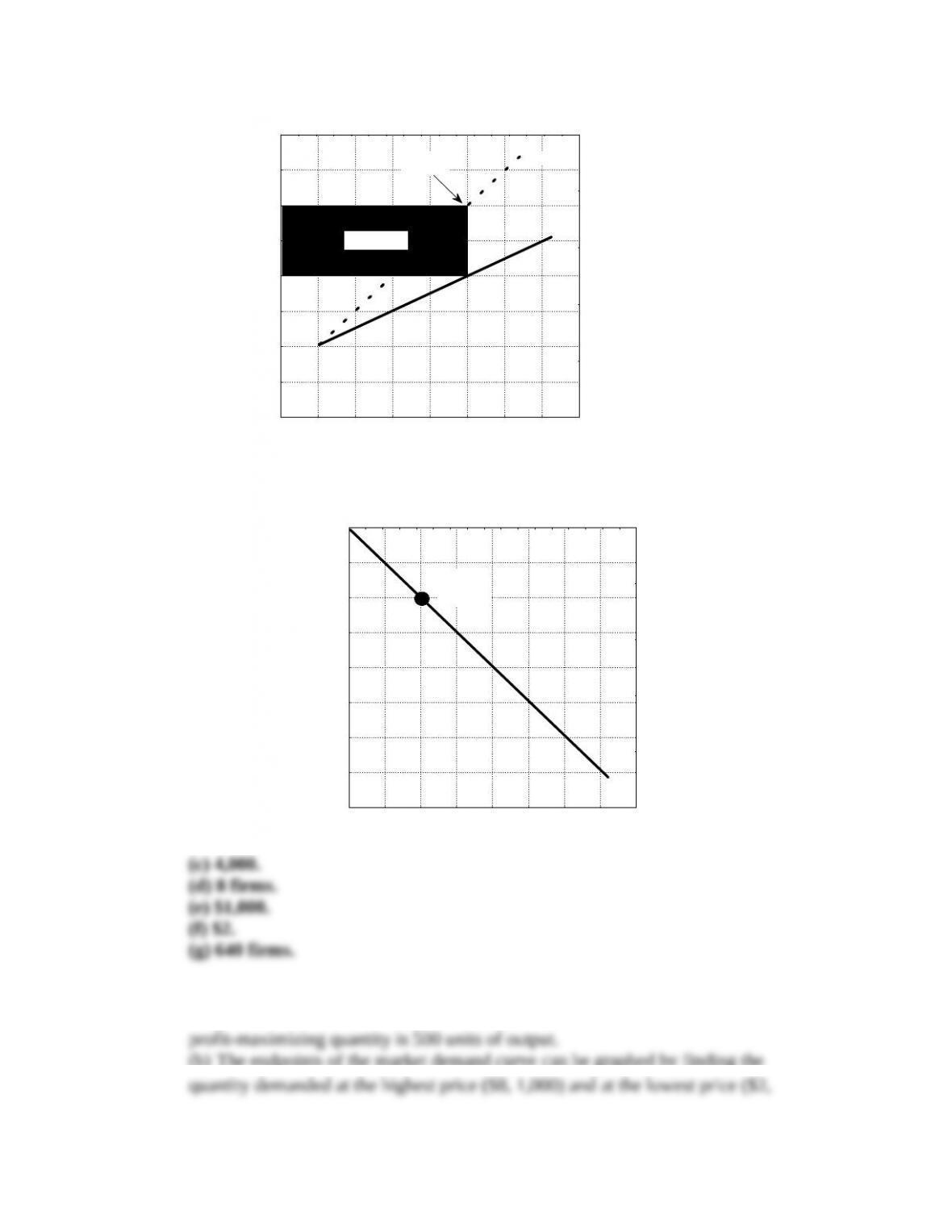
(a ) The firm
QUANTITY (fris bees per period)
P RI CE
0
1
2
3
4
5
6
7
8
0 100 200 300 400 500 6 00 700 8 00
PRO FITS
Pro fit
maximum
AT C
MC
(b) See graph below.
(b) The ma rket
QUANTITY (frisbees per period)
P RI CE
0
1
2
3
4
5
6
7
8
0 2000 4000 8 000 16 ,000 32,000 6 4,000 128 ,000 256 ,000
Market
equilibrium
price
Feedback:
(a) Profits are maximized by producing where MC = MR = P = $6. The
(b) The endpoints of the market demand curve can be graphed by finding the
6
© 2016 by McGraw-Hill Education. This is proprietary material solely for authorized instructor use. Not authorized for sale or
distribution in any manner. This document may not be copied, scanned, duplicated, forwarded, distributed, or posted on a website, in
whole or part.
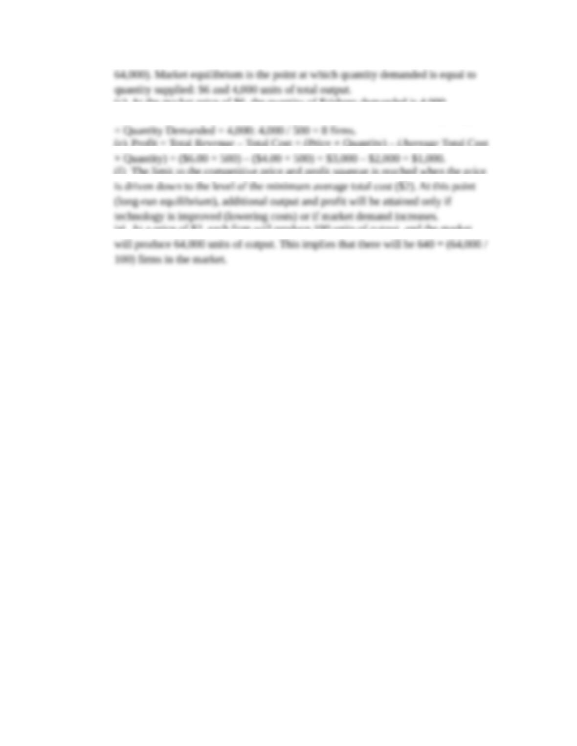
(c) At the market price of $6, the quantity of Frisbees demanded is 4,000.
(d) At a market price of $6 each firm is producing 500 Frisbees. Quantity Supplied
(e) Profit = Total Revenue – Total Cost = (Price × Quantity) – (Average Total Cost
(f) The limit to the competitive price and profit squeeze is reached when the price
(g) At a price of $2, each firm will produce 100 units of output, and the market
7
© 2016 by McGraw-Hill Education. This is proprietary material solely for authorized instructor use. Not authorized for sale or
distribution in any manner. This document may not be copied, scanned, duplicated, forwarded, distributed, or posted on a website, in
whole or part.