978-1259289903 Chapter 11 Solution Manual Part 3

subject Type Homework Help
subject Pages 8
subject Words 1669
subject Authors Bradford Jordan, Jeffrey Jaffe, Randolph Westerfield, Stephen Ross

Unlock document.

This document is partially blurred.
Unlock all pages and 1 million more documents.
Get Access
page-pf1
CHAPTER 11 B - 1
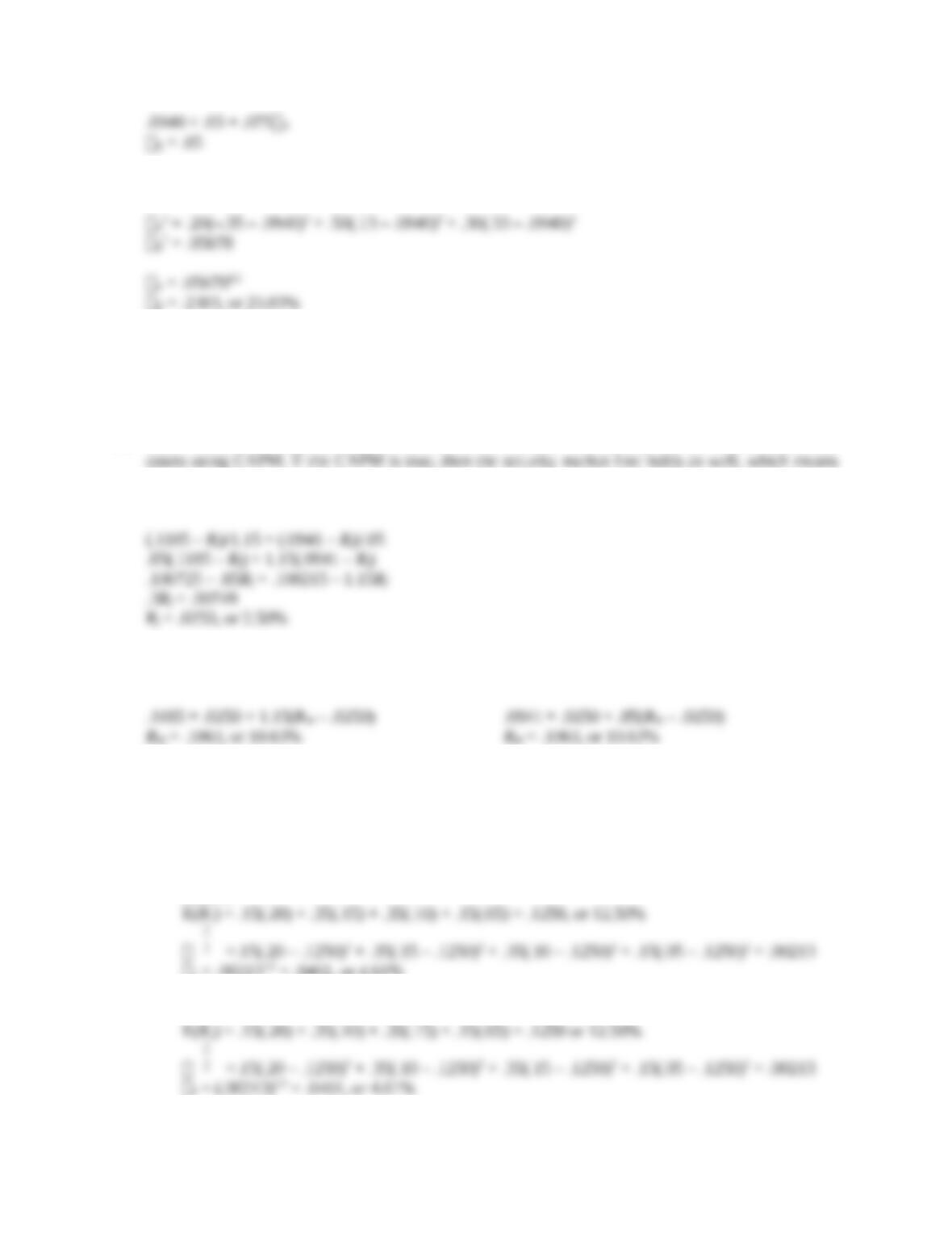
32. First, we need to find the standard deviation of the market and the portfolio, which are:
Now we can use the equation for beta to find the beta of the portfolio, which is:
Now, we can use the CAPM to find the expected return of the portfolio, which is:
Challenge
33. The amount of systematic risk is measured by the of an asset. Since we know the market risk
premium and the risk-free rate, if we know the expected return of the asset we can use the CAPM to
solve for the of the asset. The expected return of Stock I is:
E(RI) = .136, or 13.60%
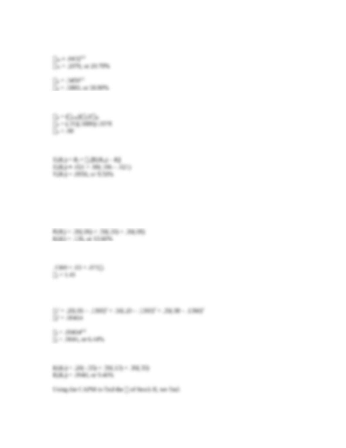
Using the CAPM to find the of Stock I, we find:
I = 1.41
The total risk of the asset is measured by its standard deviation, so we need to calculate the standard
deviation of Stock I. Beginning with the calculation of the stock’s variance, we find:
I = .0644, or 6.44%
Using the same procedure for Stock II, we find the expected return to be:
page-pf2
CHAPTER 11 B - 2
And the standard deviation of Stock II is:
II = .2383, or 23.83%
Although Stock II has more total risk than I, it has less systematic risk, since its beta is smaller than
I’s. Thus, I has more systematic risk, and II has more unsystematic and more total risk. Since
unsystematic risk can be diversified away, I is actually the “riskier” stock despite the lack of volatility
in its returns. Stock I will have a higher risk premium and a greater expected return.
34. Here we have the expected return and beta for two assets. We can express the returns of the two assets
using CAPM. If the CAPM is true, then the security market line holds as well, which means all assets
have the same risk premium. Setting the reward-to-risk ratios of the assets equal to each other and
solving for the risk-free rate, we find:
Now using CAPM to find the expected return on the market with both stocks, we find:
RM = .1063, or 10.63% RM = .1063, or 10.63%
35. a. The expected return of an asset is the sum of each return times the probability of that return
occurring. To calculate the standard deviation, we first need to calculate the variance. To find the
variance, we find the squared deviations from the expected return. We then multiply each
possible squared deviation by its probability, and then add all of these up. The result is the
variance. So, the expected return and standard deviation of each stock are:
Asset 1:
1 = .002131/2 = .0461, or 4.61%
Asset 2:
page-pf3
CHAPTER 11 B - 3
Asset 3:
E(R3) = .15(.05) + .35(.10) + .35(.15) + .15(.20) = .1250 or 12.50%
2
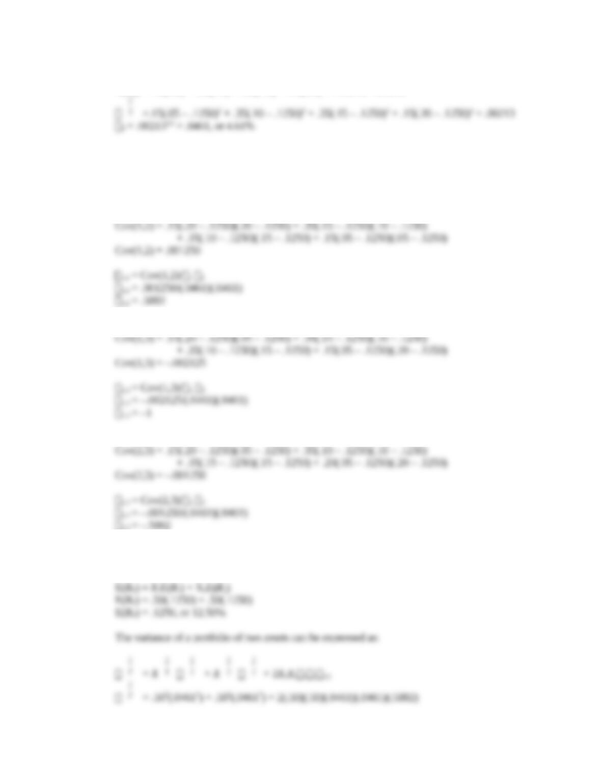
b. To find the covariance, we multiply each possible state times the product of each assets deviation
from the mean in that state. The sum of these products is the covariance. The correlation is the
covariance divided by the product of the two standard deviations. So, the covariance and
correlation between each possible set of assets are:
Asset 1 and Asset 2:
Asset 1 and Asset 3:
Asset 2 and Asset 3:
2,3 = .5882
c. The expected return of the portfolio is the sum of the weight of each asset times the expected
return of each asset, so, for a portfolio of Asset 1 and Asset 2:
page-pf4
CHAPTER 11 B - 4
2
P
= .0016875
And the standard deviation of the portfolio is:
P = .0411, or 4.11%
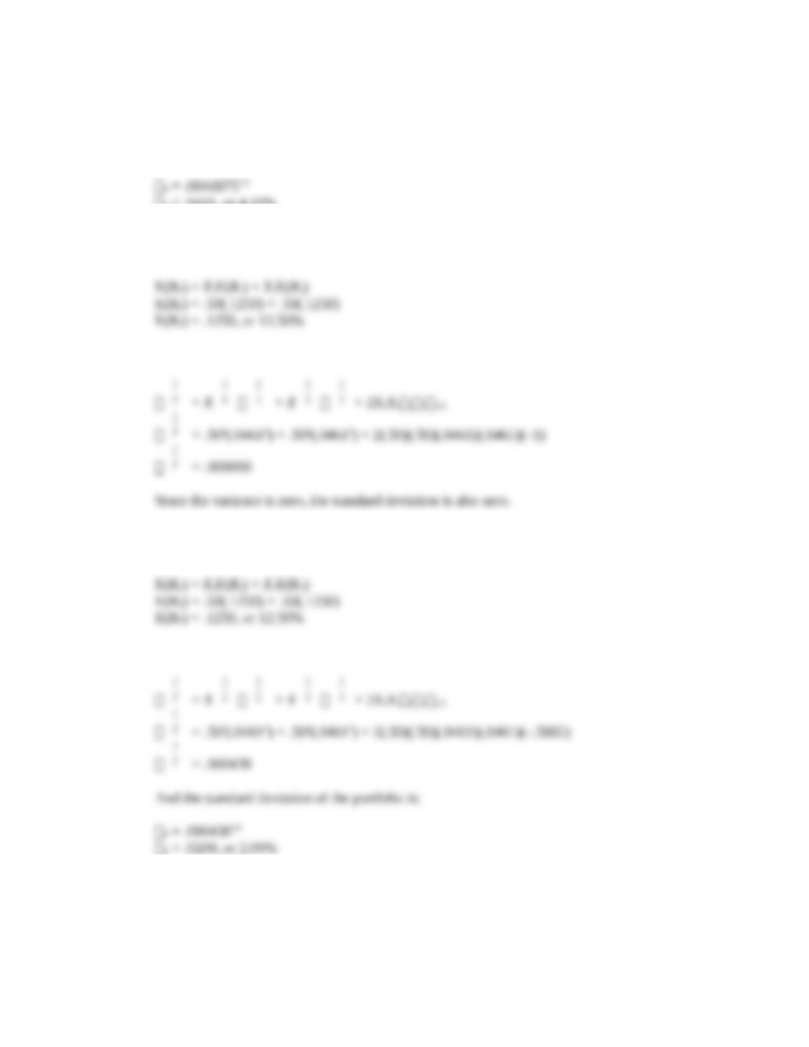
d. The expected return of the portfolio is the sum of the weight of each asset times the expected
return of each asset, so, for a portfolio of Asset 1 and Asset 3:
The variance of a portfolio of two assets can be expressed as:
e. The expected return of the portfolio is the sum of the weight of each asset times the expected
return of each asset, so, for a portfolio of Asset 2 and Asset 3:
The variance of a portfolio of two assets can be expressed as:
2
2
2
2
2
f. As long as the correlation between the returns on two securities is below 1, there is a benefit to
diversification. A portfolio with negatively correlated stocks can achieve greater risk reduction
than a portfolio with positively correlated stocks, holding the expected return on each stock
constant. Applying proper weights on perfectly negatively correlated stocks can reduce portfolio
variance to 0.
page-pf5
CHAPTER 11 B - 5
probability of that return occurring. So, the expected return of each stock is:
E(RA) = .20(.08) + .60(.12) + .20(.46)
E(RA) = .1480, or 14.80%
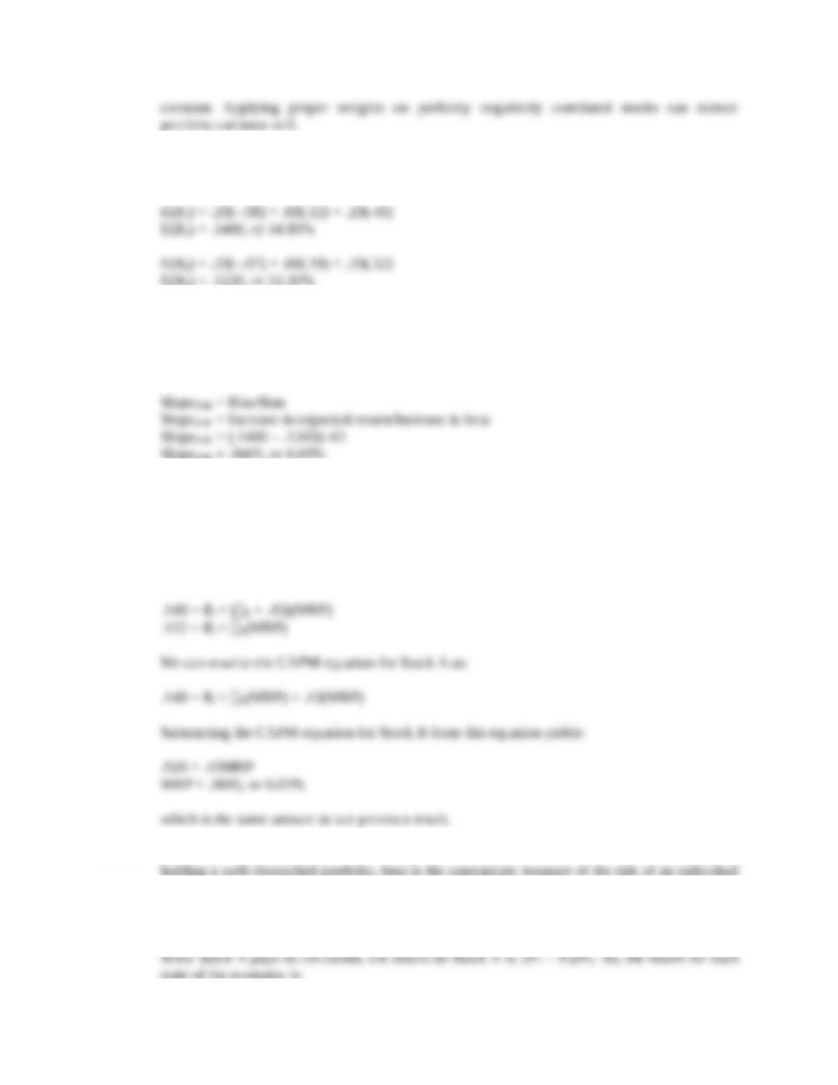
b. We can use the expected returns we calculated to find the slope of the Security Market Line. We
know that the beta of Stock A is .43 greater than the beta of Stock B. Therefore, as beta increases
by .43, the expected return on a security increases by .026 (= .1480 .1220). The slope of the
security market line (SML) equals:
SlopeSML = Rise/Run
SlopeSML = Increase in expected return/Increase in beta
Since the market’s beta is 1 and the risk-free rate has a beta of zero, the slope of the Security
Market Line equals the expected market risk premium. So, the expected market risk premium
must be 6.05 percent.
We could also solve this problem using CAPM. The equations for the expected returns of the two
stocks are:
.148 = Rf + (B + .43)(MRP)
a well-diversified portfolio, beta is the appropriate measure of the risk of an individual security.
To assess the two stocks, we need to find the expected return and beta of each of the two
securities.
Stock A:
Since Stock A pays no dividends, the return on Stock A is: (P1 P0)/P0. So, the return for each
state of the economy is:
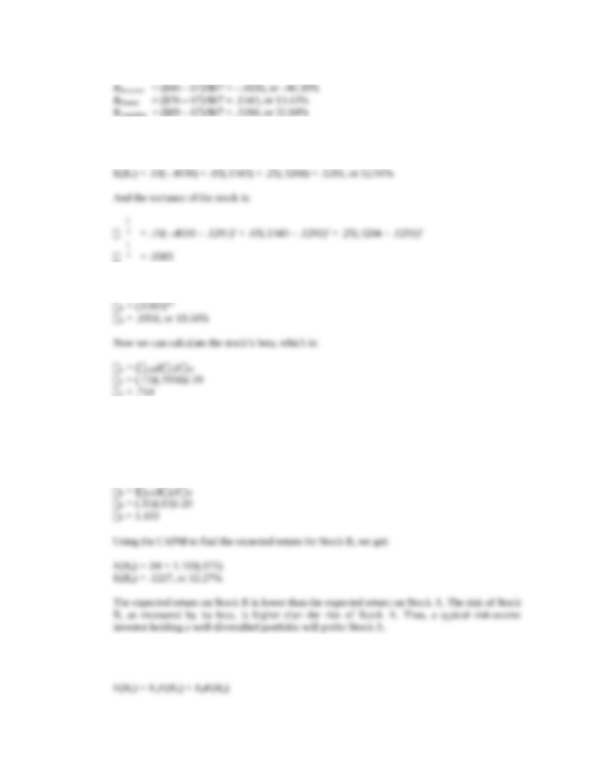
RRecession = ($40 67)/$67 = .4030, or 40.30%
page-pf6
CHAPTER 11 B - 6
RNormal = ($76 67)/$67 = .1343, or 13.43%
probability of that return occurring. So, the expected return of the stock is:
E(RA) = .10(.4030) + .65(.1343) + .25(.3284) = .1291, or 12.91%
A = (.0383)1/2
A = .1956, or 19.56%
For Stock B, we can directly calculate the beta from the information provided. So, the beta for
Stock B is:
Stock B:
B = (B,M)(B)/M
B = (.35)(.63)/.20
return of each asset, so:
E(RP) = XAE(RA) + XBE(RB)
E(RP) = .70(.1291) + .30(.1227)
page-pf7
CHAPTER 11 B - 7
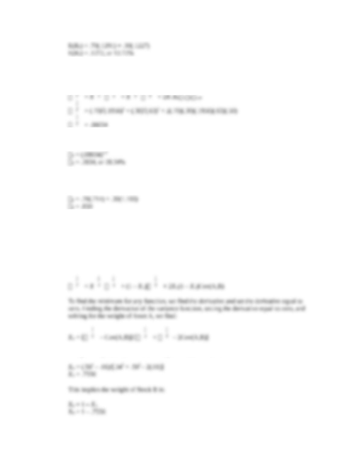
variance of the portfolio is:
2
P
= X
2
A
2
A
+ X
2
B
2
B
+ 2XAXBABA,B
2
P
= (.70)2(.1956)2 + (.30)2(.63)2 + 2(.70)(.30)(.1956)(.63)(.50)
2
P = (.08034)1/2
P = .2834, or 28.34%
of the portfolio is:
P = .70(.714) + .30(1.103)
P = .830
38. a. The variance of a portfolio of two assets equals:
2
P
= X
2
A
2
A
+ X
2
B
2
B
+ 2XAXBCov(A,B)
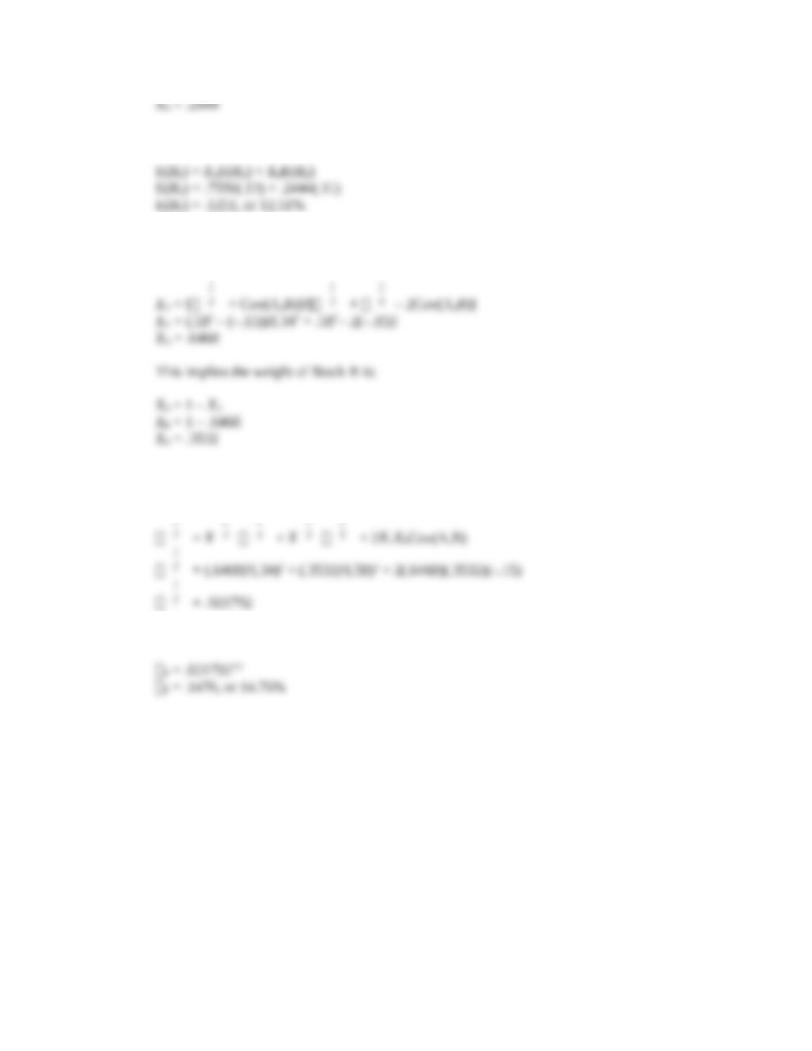
Since the weights of the assets must sum to one, we can write the variance of the portfolio as:
2
P
= X
2
A
2
A
+ (1 XA)
2
B
+ 2XA(1 XA)Cov(A,B)
XA = (.582 .01)/[.342 + .582 2(.01)]
XA = .7556
page-pf8
CHAPTER 11 B - 8
E(RP) = XAE(RA) + XBE(RB)
E(RP) = .7556(.13) + .2444(.11)
E(RP) = .1251, or 12.51%
XA = [
2
B
+ Cov(A,B)]/[
2
A
+
2
B
2Cov(A,B)]
XA = (.582 (.15))/[.342 + .582 2(.15)]
2
P
= X
2
A
2
A
+ X
2
B
2
B
+ 2XAXBCov(A,B)
2
P
= (.6468)2(.34)2 + (.3532)2(.58)2 + 2(.6468)(.3532)(.15)
2
P = .0217921/2
P = .1476, or 14.76%

Trusted by Thousands of
Students

Here are what students say about us.

Copyright ©2022 All rights reserved. | CoursePaper is not sponsored or endorsed by any college or university.