20. a. We have a special case where the portfolio is equally weighted, so we can sum the returns of
each asset and divide by the number of assets. The expected return of the portfolio is:
b. We need to find the portfolio weights that result in a portfolio with a of .50. We know the of
the risk-free asset is zero. We also know the weight of the risk-free asset is one minus the weight
of the stock since the portfolio weights must sum to one, or 100 percent. So:
And, the weight of the risk-free asset is:
c. We need to find the portfolio weights that result in a portfolio with an expected return of 10
percent. We also know the weight of the risk-free asset is one minus the weight of the stock since
the portfolio weights must sum to one, or 100 percent. So:
So, the of the portfolio will be:
d. Solving for the of the portfolio as we did in part a, we find:
borrowing at the risk-free rate to buy more of the stock.
21. We know that the reward-to-risk ratios for all assets must be equal (See Question 19). This can be
expressed as:
The numerator of each equation is the risk premium of the asset, so:
22. a. We need to find the return of the portfolio in each state of the economy. To do this, we will
multiply the return of each asset by its portfolio weight and then sum the products to get the
portfolio return in each state of the economy. Doing so, we get:
b. The risk premium is the return of a risky asset, minus the risk-free rate. T-bills are often used as
the risk-free rate, so:
RPi = .0678, or 6.78%
c. The approximate expected real return is the expected nominal return minus the inflation rate, so:
Approximate expected real return = .1048 – .031
To find the exact real return, we will use the Fisher equation. Doing so, we get:
E(ri) = .0715, or 7.15%
The approximate real risk premium is the expected nominal risk premium minus the inflation
rate, so:
23. We know the total portfolio value and the investment of two stocks in the portfolio, so we can find the
weight of these two stocks. The weights of Stock A and Stock B are:
XB = .36
Since the portfolio is as risky as the market, the of the portfolio must be equal to one. We also know
the of the risk-free asset is zero. We can use the equation for the of a portfolio to find the weight
of the third stock. Doing so, we find:
1.0 = .215(.83) + .36(1.19) + XC(1.30)
Solving for the weight of Stock C, we find:
24. We are given the expected return of the assets in the portfolio. We also know the sum of the weights
of each asset must be equal to one. Using this relationship, we can express the expected return of the
portfolio as:
And the weight of Stock Y is:
The amount to invest in Stock Y is:
25. The expected return of an asset is the sum of the probability of each return occurring times the
probability of that return occurring. So, the expected return of each stock is:
E(RB) = .1190, or 11.90%
To calculate the standard deviation, we first need to calculate the variance. To find the variance, we
find the squared deviations from the expected return. We then multiply each possible squared deviation
And the standard deviation of Stock B is:
2
2
To find the covariance, we multiply the probability of each state times the product of each assets’
deviation from the mean in that state. The sum of these products is the covariance. So, the covariance
is:
And the correlation is:
26. The expected return of an asset is the sum of the probability of each return occurring times the
probability of that return occurring. So, the expected return of each stock is:
E(RK) = .0817, or 8.17%
find the squared deviations from the expected return. We then multiply each possible squared deviation
by its probability, and then add all of these up. The result is the variance. So, the variance and standard
deviation of Stock A are:
2
2
J
= .02207
J = .022071/2
J = .1486, or 14.86%
And the standard deviation of Stock B is:
2
K
=.15(.019 – .0817)2 + .60(.118 – .0817)2 + .25(.032 – .0817)2
K
2
deviation from the mean in that state. The sum of these products is the covariance. So, the covariance
Cov(J,K) = .15(–.130 – .1251)(.019 – .0817) + .60(.098 – .1251)(.118 – .0817)
+ .25(.343 – .1251)(.032 – .0817)
return of each asset, so:
E(RP) = XFE(RF) + XGE(RG)
b. The variance of a portfolio of two assets can be expressed as:
2
P
= X
2
F
2
F
+ X
2
G
2
G
+ 2XFXG FGF,G
P
2
2
P
E(RP) = XAE(RA) + XBE(RB)
E(RP) = .40(.10) + .60(.14)
2
P
= X
2
A
2
A
+ X
2
B
2
B
+ 2XAXBABA,B
P
2
2
P
= .207401/2
= .4554, or 45.54%
return of each asset, so:
E(RP) = XAE(RA) + XBE(RB)
E(RP) = .40(.10) + .60(.14)
The variance of a portfolio of two assets can be expressed as:
2
P
= X
2
A
2
A
+ X
2
B
2
B
+ 2XAXBABA,B
P
2
2
P
= .101991/2
= .3194, or 31.94%
29. a. (i) Using the equation to calculate beta, we find:
I = (I,M)(I)/M
.85 = (I,M)(.36)/.19
I = (I,M)(I)/M
1.35 = (.38)(I)/.19
I = .68
I = (I,M)(I)/M
I = (.57)(.42)/.19
Firm A:
E(RA) = Rf + A[E(RM) – Rf]
E(RA) = .03 + .85(.12 – .03)
E(RA) = .1065, or 10.65
However, the expected return on Firm A’s stock given in the table is 11 percent. Therefore, Firm
A’s stock is underpriced, and you should buy it.
Firm B:
E(RB) = Rf + B[E(RM) – Rf]
E(RB) = .03 + 1.35(.12 – .03)
E(RB) = .1515, or 15.15%
B’s stock is overpriced, and you should sell it.
SlopeCML = [E(RM) – Rf]/M
SlopeCML = (.11 – .032)/.19
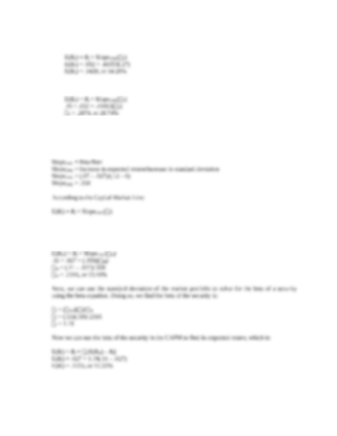
E(RP) = Rf + SlopeCML(P)
E(RP) = Rf + SlopeCML(P)
.15 = .032 + .41053(P)
31. First, we can calculate the standard deviation of the market portfolio using the Capital Market Line
(CML). We know that the risk-free asset has a return of 2.7 percent and a standard deviation of zero
and the portfolio has an expected return of 7 percent and a standard deviation of 12 percent. These two
points must lie on the Capital Market Line. The slope of the Capital Market Line equals:
SlopeCML = Rise/Run
Since we know the expected return on the market portfolio, the risk-free rate, and the slope of the
Capital Market Line, we can solve for the standard deviation of the market portfolio which is:
E(RM) = Rf + SlopeCML(M)
.11 = .027 + (.358)(M)