Chapter 06 – Bonds, Bond Prices, and the Determination of Interest Rates
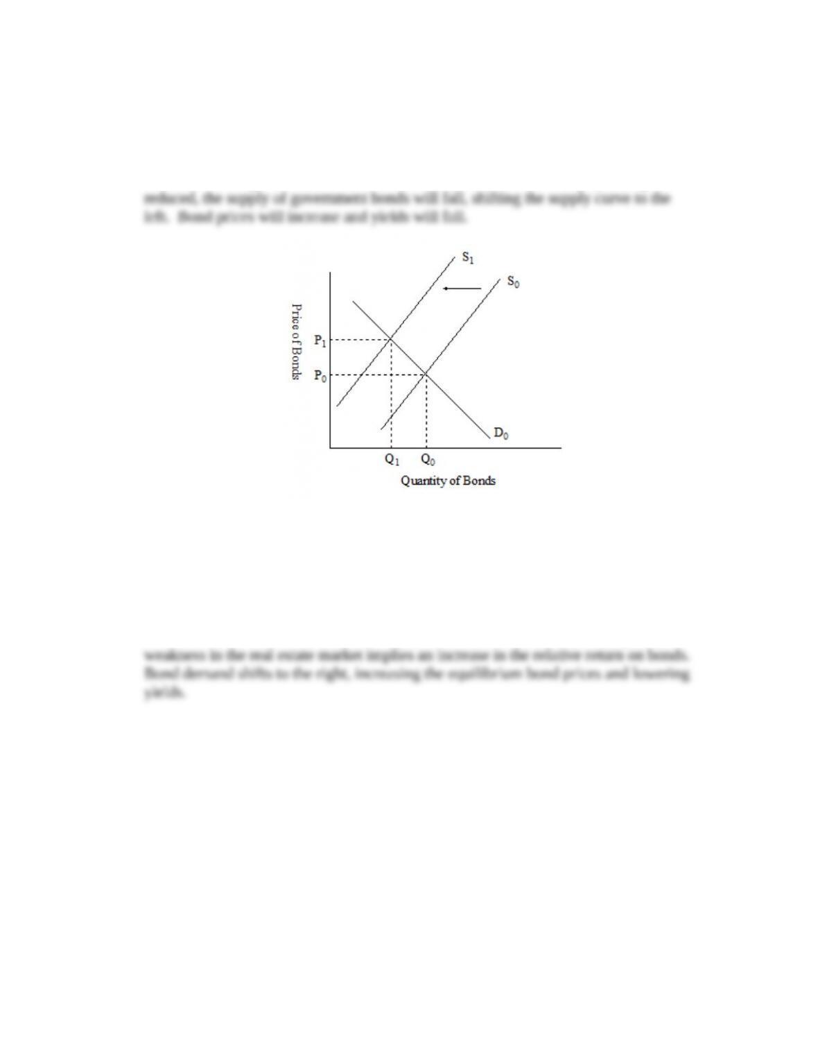
1. Suppose that a sustainable peace is reached around the world, reducing military
spending by the U.S. Government. How would you expect this development to
affect the U.S. bond market? (LO3)
Answer: As the government’s need to issue bonds to finance military spending is
2. Use the model of supply and demand for bonds to determine the impact on bond
prices and yields of expectations that the real estate market is going to weaken. (LO3)
Answer: If we think of real estate as an alternative investment to bonds, expected
6-1
Copyright © 2015 McGraw-Hill Education. All rights reserved. No reproduction or distribution without the prior written consent of
McGraw-Hill Education.

Chapter 06 – Bonds, Bond Prices, and the Determination of Interest Rates
3. *Suppose there is an increase in investors’ willingness to hold bonds at a given price.
Use the model of the demand for and supply of bonds to show that the impact on the
equilibrium bond price depends on how sensitive the quantity supplied of bonds is to
the bond price. (LO3)
Answer: The sensitivity of bond supply to changes in the price of bonds is reflected in
4. Under what circumstances would purchase of a Treasury Inflation Protected Security
(TIPS) from the U.S. government be virtually risk free? (LO4)
Answer: Purchasing a Treasury Inflation Protected Security (TIPS) would be virtually
6-2
Copyright © 2015 McGraw-Hill Education. All rights reserved. No reproduction or distribution without the prior written consent of
McGraw-Hill Education.
Price of Bonds
Quantity of Bonds
D0
D1
S
P0
P1
Price of Bonds
Quantity of Bonds
D0
D1
S
P0
P1
Chapter 06 – Bonds, Bond Prices, and the Determination of Interest Rates
5. In the wake of the financial crisis of 2007-2009, negative connotations often
surrounded the term “mortgage-backed security”. What arguments could you make
to convince someone that they may have benefitted from the growth in securitization
over the past 30 years? (LO3)
Answer: If the person you are trying to convince is a borrower, they may have
received a lower mortgage interest rate due to the increased liquidity provided by
Data Exploration
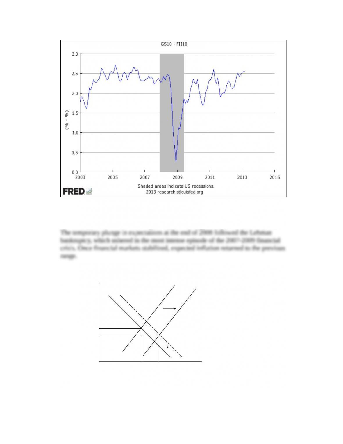
1. Graph investors’ long-term expected inflation rate since 2003 by subtracting from the
10-year U.S. Treasury bond yield (FRED code: GS10) the yield on 10-year Treasury
Inflation Protected Securities (FRED code: FII10). Do these market-based inflation
expectations appear stable? Did the financial crisis of 2007-2009 affect these
expectations? (LO4) (Hints: At the FRED Web site, click on “Data Tools” and then
“Create Your Own Graph.” In the search box below the “Settings” heading, type in
GS10. Then select “Add Data Series,” highlight the “Line 1” button, and then type
“FII10” (without the quotes) into the search box. Set the Observation Date Range to
start in January 2003. In the formula box, type “a – b” (without the quotes) to graph
the difference between the two series. Then select “Redraw Graph.”)
Answer: The indicated data plot is:
6-3
Copyright © 2015 McGraw-Hill Education. All rights reserved. No reproduction or distribution without the prior written consent of
McGraw-Hill Education.
Chapter 06 – Bonds, Bond Prices, and the Determination of Interest Rates
With the exception of the downward spike in late 2008, inflation expectations by this
measure appear stable, fluctuating mostly in the range of 2.0 percent to 2.5 percent.
6-4
Copyright © 2015 McGraw-Hill Education. All rights reserved. No reproduction or distribution without the prior written consent of
McGraw-Hill Education.
Price of Bonds
Quantity of Bonds
D0D1
S0
P0
P1
S1
Q0Q1
Chapter 06 – Bonds, Bond Prices, and the Determination of Interest Rates
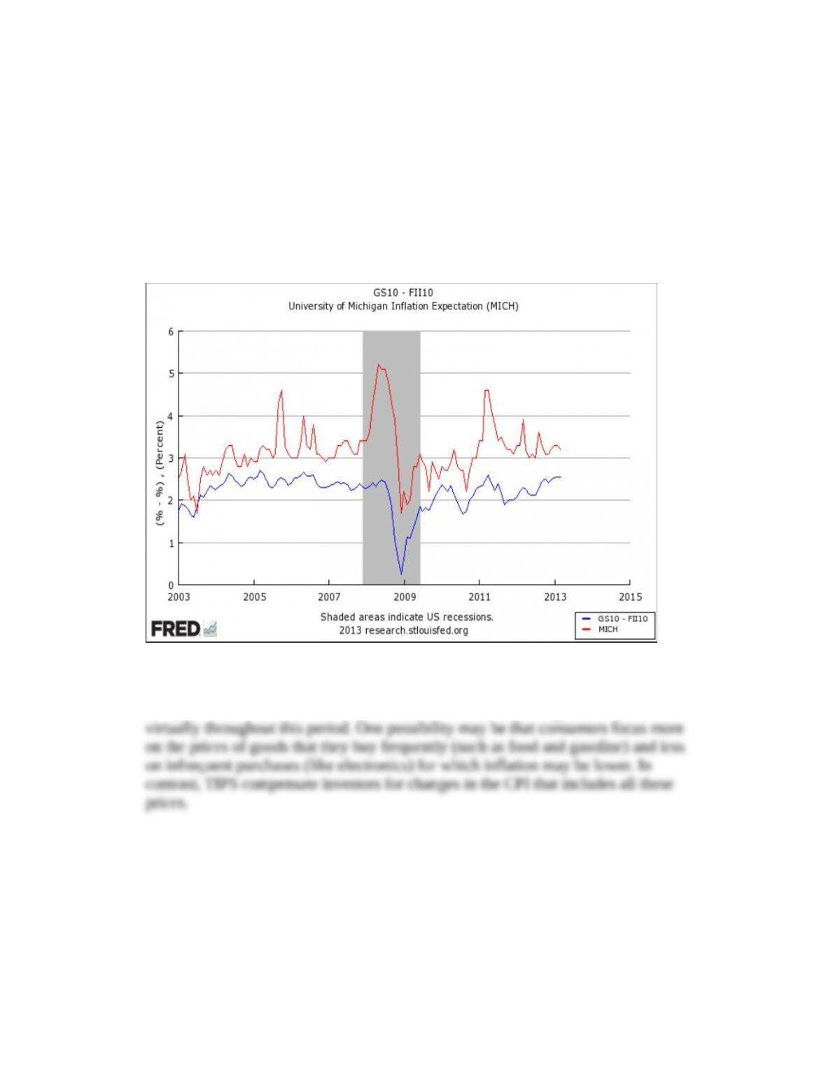
2. Compare long-run market expectations of inflation with a consumer survey measure
of one-year-ahead inflation expectations. Starting with the graph from Data
Exploration Problem 1, add as a second line the University of Michigan survey
measure of inflation expectations (FRED code: MICH) Why might these measures
differ systematically? (LO4) (Hints: Starting with the graph from question 1, select
“Add Data Series” and add a second line for the University of Michigan survey
Return to “Line 1” and select “Copy to All Lines” next to the Observation Date
Range and then “Redraw Graph.”)
Answer: The indicated data plot is:
We should not expect that one-year ahead consumer inflation expectations match
10-year-ahead investor inflation expectations. However, it is interesting that
consumer short-term inflation expectations exceed investor long-term expectations
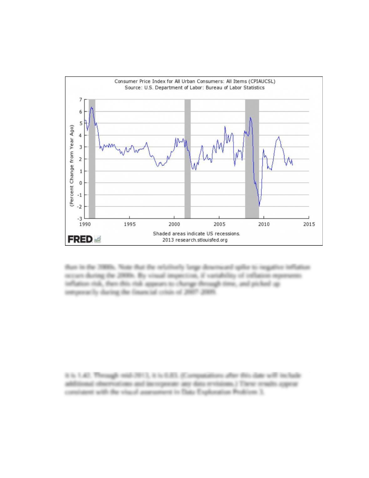
3. How does the variability of annual inflation – an indicator of inflation risk – change
over time? Graph the percent change from a year ago of the consumer price index
(FRED code: CPIAUCSL) since1990 and visually compare the decades of the 1990s,
the 2000s, and the period that began in 2010. (LO4) (Hints: At the FRED Web site,
select “Data Tools” and then “Create Your Own Graph.” In the search box below the
“Settings” heading, enter the identifier for the consumer price index (FRED code:
CPIAUCSL). Set the “Observation Date Range” to start in 1990, select “Percent
6-5
Copyright © 2015 McGraw-Hill Education. All rights reserved. No reproduction or distribution without the prior written consent of
McGraw-Hill Education.
Chapter 06 – Bonds, Bond Prices, and the Determination of Interest Rates
Change from Year Ago” from the “Units” dropdown box, and then “Redraw
Graph.”)
Answer: The data plot is:
After inflation declines to around 3 percent in the early 1990s, it appears less variable
4. Download the data from the graph you produced in Data Exploration Problem 3.
Calculate the standard deviation of the annual inflation rate for the three time periods
and compare these results against your visual assessment from Data Exploration
Problem 3. (LO4) (Hint: Above the graph, select “Download Data in Graph” to
create a spreadsheet with the inflation data. Use the spreadsheet function STDEV to
calculate the standard deviation of annual inflation for each time period.)
Answer: The standard deviation from 1990 through 1999 is 1.13; from 2000 to 2009,
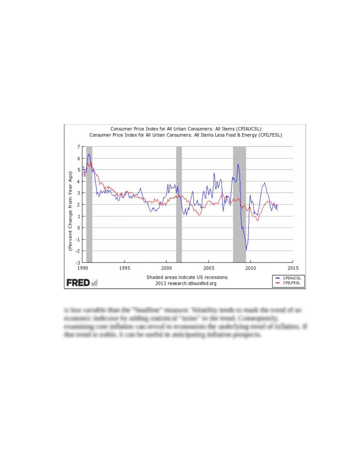
5. Economists sometimes exclude food and energy prices from the “headline” consumer
price index and use the resulting “core” price measure to assess inflation prospects.
For the period since 1990, plot on one graph the percent change from a year ago of
6-6
Copyright © 2015 McGraw-Hill Education. All rights reserved. No reproduction or distribution without the prior written consent of
McGraw-Hill Education.
Chapter 06 – Bonds, Bond Prices, and the Determination of Interest Rates
the consumer price index (FRED code: CPIAUCSL) and the percent change from a
year ago of the consumer price index excluding food and energy (FRED code:
CPILFESL) Visually compare the variability of these two measures of inflation. Why
might ex-food-and-energy inflation be a better predictor of future inflation? (LO4)
(Hint: Starting with the graph in Data Exploration Problem 3, select “Add Data
Series,” add the core CPI code (FRED code: CPILFESL) in the search box, set the
“Observation Date Range” to start in January 1990, select “Percent Change from
Year Ago” from the “Units” dropdown box, and then “Redraw Graph.”)
Answer: The data plot is:
Because food and energy prices are relatively volatile, the “core” measure of inflation
* indicates more difficult problems
6-7
Copyright © 2015 McGraw-Hill Education. All rights reserved. No reproduction or distribution without the prior written consent of
McGraw-Hill Education.