CHAPTER 8: INDEX MODELS
17. a.
Alpha (α) Expected excess return
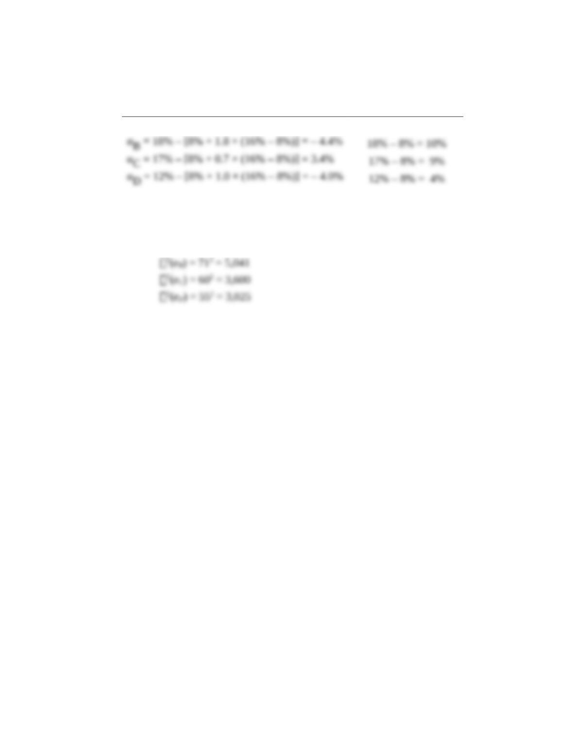
αi = ri – [rf + βi × (rM – rf ) ] E(ri ) – rf
αA = 20% – [8% + 1.3 × (16% – 8%)] = 1.6% 20% – 8% = 12%
Stocks A and C have positive alphas, whereas stocks B and D have
negative alphas.
The residual variances are:
2(eA ) = 582 = 3,364
8-1
CHAPTER 8: INDEX MODELS
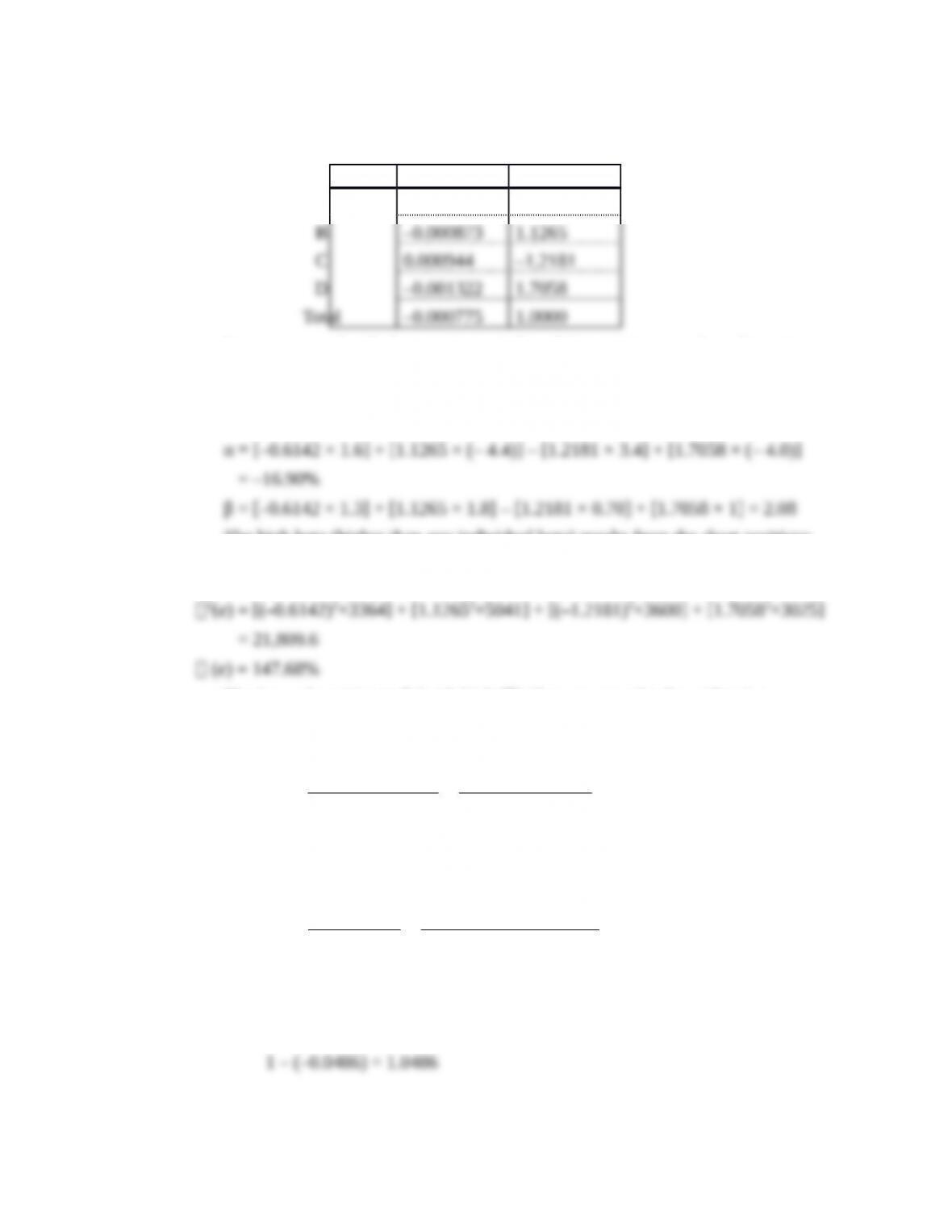
b. To construct the optimal risky portfolio, we first determine the optimal active
portfolio. Using the Treynor-Black technique, we construct the active portfolio:
A
0.000476
–0.6142
Be unconcerned with the negative weights of the positive α stocks—the entire
active position will be negative, returning everything to good order.
With these weights, the forecast for the active portfolio is:
The high beta (higher than any individual beta) results from the short positions
in the relatively low beta stocks and the long positions in the relatively high
beta stocks.
The levered position in B [with high 2(e)] overcomes the diversification
effect and results in a high residual standard deviation. The optimal risky
portfolio has a proportion w* in the active portfolio, computed as follows:
2
02 2
/ ( ) .1690 / 21,809.6 0.05124
[ ( ) ] / .08 / 23
M f M
e
wE r r
a s
s
–
= = =-
–
The negative position is justified for the reason stated earlier.
The adjustment for beta is:
0486.0
)05124.0)(08.21(1
05124.0
)β1(1
*
0
0
w
w
w
Since w* is negative, the result is a positive position in stocks with positive
alphas and a negative position in stocks with negative alphas. The position in
the index portfolio is:
1 – (–0.0486) = 1.0486
8-2
CHAPTER 8: INDEX MODELS
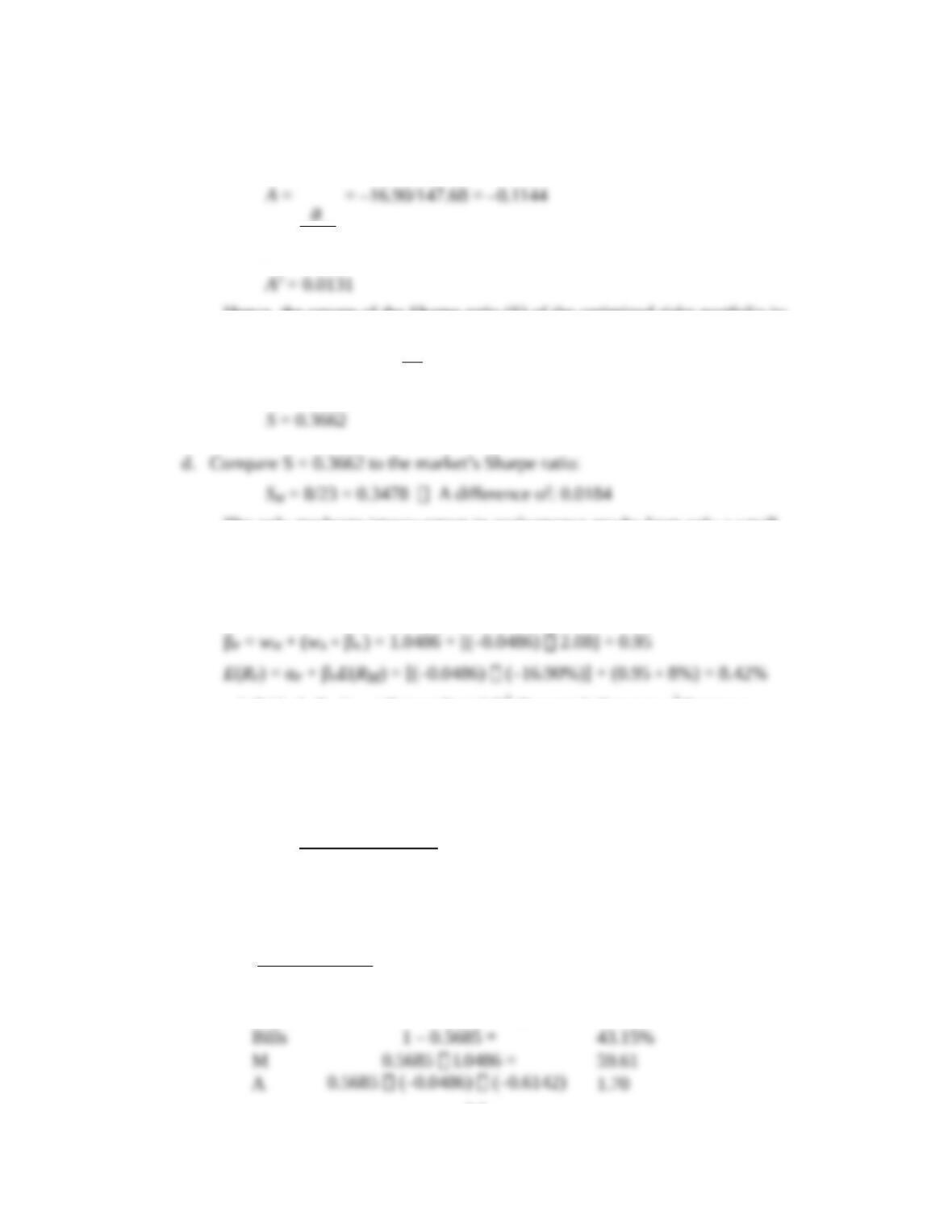
c. To calculate the Sharpe ratio for the optimal risky portfolio, we compute the
information ratio for the active portfolio and Sharpe’s measure for the market
portfolio. The information ratio for the active portfolio is computed as follows:
Hence, the square of the Sharpe ratio (S) of the optimized risky portfolio is:
1341.00131.0
23
8
2
222
ASS
M
The only moderate improvement in performance results from only a small
position taken in the active portfolio A because of its large residual variance.
e. To calculate the makeup of the complete portfolio, first compute the beta, the
mean excess return, and the variance of the optimal risky portfolio:
94.5286.809,21)0486.0()2395.0()(σσβσ 222222 PMPP e
%00.23σ
P
Since A = 2.8, the optimal position in this portfolio is:
5685.0
94.5288.201.0
42.8
y
In contrast, with a passive strategy:
5401.0
238.201.0
8
2
y
A difference of: 0.0284The final positions are
(M may include some of stocks A through D):
=
8-3
CHAPTER 8: INDEX MODELS
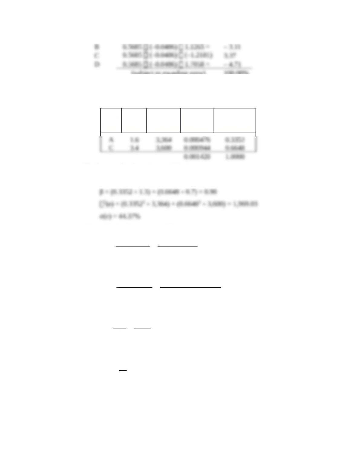
(subject to rounding error) 100.00%
18. a.If a manager is not allowed to sell short, he will not include stocks with negative
alphas in his portfolio, so he will consider only A and C:
Α2(e)
The forecast for the active portfolio is:
α = (0.3352 × 1.6) + (0.6648 × 3.4) = 2.80%
The weight in the active portfolio is:
0940.0
23/8
03.969,1/80.2
σ/)(
)(σ/α
22
2
0
MM
RE
e
w
Adjusting for beta:
0931.0
]094.0)90.01[(1
094.0
w)1(1
w
*w
0
0
The information ratio of the active portfolio is:
2.80 0.0631
( ) 44.37
Ae
a
s
= = =
Hence, the square of the Sharpe ratio is:
2
2 2
80.0631 0.1250
23
Sæ ö
= + =
ç ÷
è ø
Therefore: S = 0.3535
8-4

CHAPTER 8: INDEX MODELS
When short sales are allowed (Problem 17), the manager’s Sharpe ratio is
8-5

CHAPTER 8: INDEX MODELS
2 2 2 2 2 2
(1 0.0931) (0.0931 0.9) 0.99
( ) ( ) (0.0931 2.8%) (0.99 8%) 8.18%
( ) (0.99 23) (0.0931 1969.03) 535.54
23.14%
P M A A
P P P M
P P M P
P
w w
E R E R
e
b b
a b
s b s s
s
With A = 2.8, the optimal position in this portfolio is:
5455.0
54.5358.201.0
18.8
y
The final positions in each asset are:
Bills 1 – 0.5455 = 45.45%
b. The mean and variance of the optimized complete portfolios in the
unconstrained and short-sales constrained cases, and for the passive strategy
are:
E(RC )
2
σC
Unconstrained 0.5685 × 8.42% = 4.79 0.56852 × 528.94 = 170.95
The utility levels below are computed using the formula:
2
σ005.0)(
CC
ArE
Unconstrained 8% + 4.79% – (0.005 × 2.8 × 170.95) = 10.40%
8-6
CHAPTER 8: INDEX MODELS
19. All alphas are reduced to 0.3 times their values in the original case. Therefore, the
relative weights of each security in the active portfolio are unchanged, but the alpha
2
02 2
/ ( ) 0.0507 / 21,809.6 0.01537
( ) / 0.08 / 23
M f M
e
wE r r
a s
s
The negative position is justified for the reason given earlier.
The adjustment for beta is:
0151.0
)]01537.0()08.21[(1
01537.0
)β1(1
*
0
0
w
w
w
Since w* is negative, the result is a positive position in stocks with positive alphas
and a negative position in stocks with negative alphas. The position in the index
portfolio is: 1 – (–0.0151) = 1.0151
To calculate the Sharpe ratio for the optimal risky portfolio we compute the information
5.07
( ) 147.68e
a
s
–
=
Hence, the square of the Sharpe ratio of the optimized risky portfolio is:
Compare this to the market’s Sharpe ratio: SM =
8%
23%
= 0.3478
The difference is: 0.0017
Note that the reduction of the forecast alphas by a factor of 0.3 reduced the squared
information ratio and the improvement in the squared Sharpe ratio by a factor of:
20. If each of the alpha forecasts is doubled, then the alpha of the active portfolio will
also double. Other things equal, the information ratio (IR) of the active portfolio
8-7

CHAPTER 8: INDEX MODELS
8-8
CHAPTER 8: INDEX MODELS
CFA PROBLEMS
1. The regression results provide quantitative measures of return and risk based on
monthly returns over the five-year period.
β for ABC was 0.60, considerably less than the average stock’s β of 1.0. This
indicates that, when the S&P 500 rose or fell by 1 percentage point, ABC’s return
on average rose or fell by only 0.60 percentage point. Therefore, ABC’s systematic
β for XYZ was somewhat higher, at 0.97, indicating XYZ’s return pattern was very
similar to the β for the market index. Therefore, XYZ stock had average systematic
risk for the period examined. Alpha for XYZ was positive and quite large,
The effects of including one or the other of these stocks in a diversified portfolio
may be quite different. If it can be assumed that both stocks’ betas will remain
stable over time, then there is a large difference in systematic risk level. The betas
obtained from the two brokerage houses may help the analyst draw inferences for
These stocks appear to have significantly different systematic risk characteristics. If
these stocks are added to a diversified portfolio, XYZ will add more to total volatility.
8-9
CHAPTER 8: INDEX MODELS
c
8-10